A Waste-Efficient Algorithm for Single-Droplet Sample Preparation on Microfluidic Chips

Marek Chrobak; Miguel Coviello Gonzalez

REVIEW 4 major objections 5 minor 10 references

A Waste-Efficient Algorithm for Single-Droplet Sample Preparation on Microfluidic Chips

T0 review · 4 major / 5 minor · reviewed 2026-08-14 · deepseek-v4-flash

Challenge this review Re-run · record.json Download PDF Read on arXiv ↗ Review JSON

Pith's one-line read The paper proves RPRIS, a mixing-graph algorithm for single-droplet sample preparation, produces at most (d+γ)/2 + 2 waste droplets, about half the baseline Min-Mix's d.

desk verdict RPRIS is a credible new single-droplet mixing algorithm whose provable waste guarantee roughly halves Min-Mix, but the main theorem's proof leans on an unformalized Claim 1 and a +2/+4 bound inconsistency that need real fixing before publication. read the letter →

arxiv 1908.09618 v3 pith:NSK72UFK submitted 2019-08-20 cs.DS cs.DM

Miguel Coviello Gonzalez , Marek Chrobak This is my paper · ORCID

classification cs.DScs.DM

keywords microfluidicchipssamplepreparationmixinggraphswasteminimizationdroplet-basedmodelRPRISalgorithmbinaryprecisiondilution

verification ladder T0 review T1 audit T2 compute T3 formal

The pith

A machine-rendered reading of the paper's core claim, the machinery that carries it, and where it could break.

The reading

This paper proposes RPRIS (Recursive Precision Reduction with Initial Shift), an algorithm that designs mixing graphs for producing a single droplet of a target reactant concentration from pure reactant and buffer droplets, and it proves a worst-case guarantee on the number of waste droplets. The guarantee is at most (d+γ)/2 + 2 waste droplets, where d is the binary precision of the target concentration and γ counts the equal leading bits in its binary representation; Min-Mix, the standard baseline, always produces exactly d waste droplets, so RPRIS cuts the worst case roughly in half for most concentrations. The argument works by a recursive step that lowers the precision of the target by 2 while adding only one waste droplet, with at most one exceptional step that adds two, followed by an initial shift that handles concentrations outside [1/4, 3/4]. In experiments over all concentrations of precision 7, 8, 15, and 20, RPRIS averages about 50% less waste than Min-Mix and 21–25% less than DMRW; for precisions 7 and 8, where GORMA and ILP can run, it averages about 17% less than GORMA and only about 7% above ILP.

What carries the argument

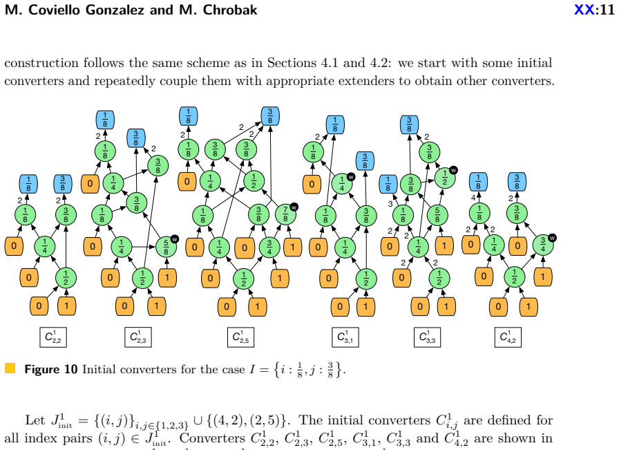
The load-bearing machinery is a set of converter graphs C^k_{i,j}, each a small mixing graph that takes i droplets of one endpoint concentration l and j of the other endpoint r (with l, r the endpoints of one of five intervals covering [1/4, 3/4]) and produces them from 0/1 inputs while emitting at most one waste droplet; four exceptional converters emit two, and the proof shows only $C^{1}$_{1,3} among them can ever be used, at most once. Recursive Precision Reduction applies the inverse linear map t_{s+1} = 4(t_s − l) to lower precision by 2 per level, then couples the recursively built graph with the appropriate converter, relabeling every concentration c as l + c/4. Initial Shift first maps targets outside [1/4, 3/4] into that interval by a shift of 2^γ or $2^{{γ−1}}$, paying at most γ−σ waste droplets. The whole construction is linear-time in the output graph, and output graphs have size O($d^{2}$).

What would settle it

Run RPRIS on all target concentrations with precision d for d = 7, 8, ..., 20 and record the converters used in each recursion; finding any target for which $C^{1}$_{6,1} or $C^{1}$_{3,2} appears would refute Lemma 2(iii) and with it Theorem 1. Independently, trace every source-to-sink path in the converter diagrams of Figures 7–11 and check that each labeled output concentration equals the average of its two input labels; one mislabeled edge would invalidate the converter construction on which the bound rests.

Watch

Extended reading notes

Core claim

The central claim is Theorem 1: for any single-droplet target t, the mixing graph produced by RPRIS has at most (d+γ)/2 + 2 waste droplets, where d = prec(t) and γ is the number of equal leading bits in the binary representation of t, not counting the least-significant 1. Because Min-Mix always produces exactly d waste droplets, this gives a worst-case waste of about half that of Min-Mix for almost all concentrations; for t in [1/4, 3/4] the bound is d/2 + O(1), whereas DMRW's worst case in the same range is still d − O(1). The proof counts sink nodes in the constructed graph: the initial shift contributes at most γ−σ waste droplets, and the recursive reduction builds a graph with at most d0/2 + 3 sinks, using the fact that every RPR step but at most one contributes only one waste sink.

Load-bearing premise

The load-bearing premise is that the case analysis in Claim 1 is complete: no reachable state of the RPR recursion ever requires the two-waste converters $C^{1}$_{6,1} or $C^{1}$_{3,2} (or their symmetric counterparts), and the converter diagrams in Figures 7–11 are all correct.

Editorial extensions

If this is right

For every single-droplet target with precision d, RPRIS produces at most (d+γ)/2 + 2 waste droplets, so the worst-case guarantee is about half that of Min-Mix for almost all concentrations.
For target concentrations in [1/4, 3/4], the waste bound is d/2 + O(1), a strict worst-case improvement over DMRW's d − O(1) in that range.
Because the optimum waste is at least γ + 1, RPRIS can be read as matching the leading γ term and paying roughly half of the remaining d − γ bits in waste.
The algorithm runs in time linear in the size of the mixing graph it outputs, and the output graph has O(d^2) nodes, so the construction is practical for the precisions tested.
On all tested concentrations of precision 7, 8, 15, and 20, RPRIS is never worse than Min-Mix or REMIA, is worse than DMRW on fewer than 3.5% of precision-20 concentrations, and stays within about 7% of ILP, which is doubly exponential.

Reading between the lines

Editorial extensions of the paper, not claims the author makes directly.

The same precision-reduction template could be pushed further: if a converter family were found that reduces precision by k while adding fewer than k waste droplets per level, the waste bound could drop below d/2 + O(1), potentially approaching the γ + 1 lower bound; the paper does not construct such a family.
Claim 1's reachability statement is checkable by exhaustive simulation: running RPRIS on every target of precision up to, say, 20 and recording which converters are invoked would either confirm the informal 'not enough reactant' arguments or produce a counterexample that breaks Theorem 1.
The waste measure (d, γ) may transfer to reactant minimization or to multi-droplet target sets; the paper itself notes that recursive precision reduction might adapt to reactant minimization, but no such algorithm is given.

Share X Bluesky LinkedIn Reddit HN

Signed reviews

No signed human review yet.

Editorial analysis

A structured set of objections, weighed in public.

Desk editor's note, referee report, and a circularity audit.

Desk Editor's Note

read the letter

You should know this paper first for what it actually adds: RPRIS is a new recursive algorithm for single-droplet sample preparation, and the (d, gamma) worst-case measure is a genuinely useful way to state performance. The construction — recursive precision reduction plus an initial shift, with converters that mostly waste one droplet — is new, and the claimed bound of about 1/2(d+gamma) is a real improvement over Min-Mix's exact d. The experimental comparison is also honestly done: it sweeps all concentrations at several precisions, reports averages and worst-case percentages, and shows 21-25% less waste than DMRW and roughly half of Min-Mix, while staying only about 7% above ILP for small d. That is a solid engineering contribution.

Where the paper is soft is exactly where the stress-test note lands. Theorem 1's proof reduces to Lemma 2, and Lemma 2's part (iii) depends on Claim 1, which rules out converters C^1_{6,1} and C^1_{3,2} by interval cases and phrases like "not enough reactant" rather than by a formal reachable-state invariant. The converter diagrams in Figures 7-11 are also not independently verified; if any of them hides an extra waste droplet, the bound could shift. I want to be fair about severity: even if Claim 1 failed, the bound would only worsen by one or two droplets — the central idea would not collapse. But as written, the proof is not airtight, and the paper's own text makes things worse by citing "1/2(d+gamma)+4" in Section 6 while Theorem 1 says +2. That inconsistency has to be fixed, not hand-waved.

The other weaknesses are minor by comparison: no code or raw data is shipped, and the experimental figures are smoothed, so the 17% vs GORMA claim is hard to reproduce from the PDF alone. The source-count monotonicity used to limit C^1_{1,3} to one use is plausible but unstated; it deserves a short formal justification.

Net: the paper is worth serious refereeing. The algorithm and measure are new, the experiments are meaningful, and the proof gap is likely patchable. A good referee will ask for a formal proof of Claim 1, a reconciliation of the +2/+4 discrepancy, and either code or a data appendix. I would not desk-reject this.

For your own choices: I would take it to a reading group, and I would cite it if I did anything in microfluidic sample preparation — the algorithm is the current practical baseline. The authors are clearly thinking hard about the right model and measure, even if the proof needs another pass.

Referee Report

4 major / 5 minor

Summary. The paper addresses the design of mixing graphs for single-droplet sample preparation in the droplet-based microfluidic model, where 1-1 mixers average pairs of droplet concentrations and the goal is to produce a target droplet of concentration t while minimizing the number of waste droplets. The authors propose RPRIS (Recursive Precision Reduction with Initial Shift): an Initial Shift maps t into [1/4, 3/4] via multiplication by a power of two, and a recursive procedure repeatedly reduces the target precision by two by mapping the current concentration through one of five overlapping intervals S1–S5; on backtracking, the graph built for the reduced target is coupled with a converter from a family C^k_{i,j} constructed in Sections 4.1–4.3. The main theoretical claim (Theorem 1) is that RPRIS produces at most 1/2(d+γ)+2 waste droplets, where d = prec(t) and γ is the length of the leading run of equal bits in the binary representation of t, compared with exactly d for Min-Mix and d−O(1) worst case for DMRW. The proof (Lemma 2) bounds the number of sink nodes of the recursively built graph by 1/2 d0 + 3 using three claims about the base graphs, the number of converters, and the number of two-waste converters; the last claim depends on an informal Claim 1.

Significance. If Theorem 1 is established, this is a meaningful advance for a problem where even the computability of the optimum is open: RPRIS is, to my knowledge, the first waste-minimization algorithm for single-droplet targets with a provable parameter-dependent worst-case bound that improves on the trivial d-waste bound of Min-Mix by a factor of about two, and the bound naturally tracks the binary structure of the target. The experimental methodology is a strength: the study exhaustively sweeps all concentrations at the tested precisions and compares against five published algorithms including the exponential-time ILP approach, and the reported findings (e.g., RPRIS is never worse than Min-Mix or REMIA on any tested concentration) are concrete and falsifiable. The authors are also appropriately candid about the limits of the analysis, noting that no super-constant lower bound on waste is known for t in [1/4, 3/4]. The paper does not ship code or machine-checked proofs, and the correctness of the converter diagrams in Figures 7–11 is assumed; this is the main source of residual risk.

major comments (4)

[Section 5, Claim 1 and Lemma 2(iii)] Claim 1, on which Lemma 2(iii) rests, is not proved rigorously. The argument for C^1_{6,1} and the three interval cases for C^1_{3,2} rely on assertions that are stated rather than derived: 'there is not enough reactant available to produce t_{s+1}' (C^1_{6,1} case); 'the only C^3_{i,j} converter with source concentration labels {3:0, 2:1} is C^3_{3,1}' together with an unverified claim about its sink labels (Case 1); 'every converter and extender in Section 4.1 adds at least the same number of source nodes with concentration label 0 as source nodes with concentration label 1' (Case 2); and 'to produce concentration 7/8, at least three reactant droplets are needed' (Case 3). Each of these statements is plausible, but none is proved from the converter constructions, and the diagrams in Figures 7–11 are not independently verified. Since Lemma 2(iii) is exactly the step that keeps the additive constant at +2 in Theorem 1, the proof of the theorem is incomplete as written; the authors should provide a formal reachability argument or a machine-checked enumeration of the converter family.
[Section 5, Lemma 2(iii), paragraph on C^1_{1,3}] The restriction that C^1_{1,3} 'can not be used more than once' is justified by the sentence 'the number of source nodes at each recursive step in the RPR process is decreasing,' but this monotonicity is asserted without proof and is not an immediate consequence of the extender rules in Section 4.3, which preserve i+j rather than the number of 0/1 source nodes of the assembled converter. A second use of C^1_{1,3} would add another two-waste converter and degrade the constant in Theorem 1, so this step requires an explicit proof or a different argument bounding the number of uses.
[Section 6 vs Section 5 (waste bound constants)] Section 6 states that the observed roughly 50% waste reduction relative to Min-Mix is 'consistently with our bound of 1/2(d+γ)+4 on waste produced by RPRIS,' whereas Theorem 1 and the proof of Lemma 2 both give 1/2(d+γ)+2. The paper therefore presents two different constants for its main quantitative claim. One of the two statements must be corrected, and if the intended bound is +4, then Theorem 1, Lemma 2, and the abstract need to be revised accordingly.
[Section 4.3 vs Section 5 (enumeration of two-waste converters)] The lists of exceptional two-waste converters disagree between sections: Section 4.3 concludes that the exceptions are C^1_{1,1}, C^1_{1,3}, C^1_{3,2}, and C^1_{1,6}, whereas Lemma 2(iii) in Section 5 enumerates C^1_{1,3}, C^1_{3,2}, and C^1_{6,1}, and Claim 1 rules out only C^1_{6,1} and C^1_{3,2}. If C^1_{1,6} is genuinely a two-waste converter, its possible use is never analyzed and the +2 bound is unsupported; if 'C^1_{1,6}' is a typo for 'C^1_{6,1}', the text should be corrected. Section 4.3 explicitly constructs C^1_{6,1} as X^1_1 • C^1_{3,2}, so the two lists cannot both be right as written.

minor comments (5)

[Section 5, Lemma 2(ii)] The claim that db ∈ {2, 3} is false: for t0 = 21/64, the chosen interval is S2 and the recursion reaches t1 = 5/16 ∈ B, giving db = 4. The needed conclusion db ≥ 2 (and hence at most 1/2 d0 − 1 converters) still holds, since db = 1 would force t_b = 1/2 and hence an earlier base case, but the stated claim should be corrected.
[Section 4.3] The parenthetical '(It is easy to prove that for these converters waste 2 cannot be avoided.)' asserts a nontrivial claim without proof; either supply the argument or remove the sentence.
[Section 1, Discussion paragraph] The probabilistic statement that for uniformly random t of precision d the waste exceeds (1/2−ε)d with probability tending to zero is stated without proof; a one-sentence derivation from the distribution of γ would make the remark self-contained.
[Section 6, Figures 12–13] The figures are smoothed using MATLAB's smooth function; since the text reports specific percentages of concentrations where RPRIS loses to DMRW or GORMA, plotting unsmoothed data or including a table of raw statistics would make the experimental claims directly verifiable.
[References] The bibliography entry for [5] prints the author names without separating spaces ('MiguelCovielloGonzalezandMarekChrobak'); the formatting should be fixed.

Circularity Check

0 steps flagged · score 0.0 of 10

No circularity: RPRIS waste bound is derived from the algorithm's own recursion and explicit converter constructions, not from a fitted parameter or self-citation.

full rationale

The central result, Theorem 1, is a worst-case bound on waste derived from the algorithm's own structure: Lemma 2 counts sink nodes from the base-case graphs, the fact that each RPR recursion step lowers precision by exactly 2, and the stated waste profiles of the explicitly constructed converters. The parameters d and gamma are defined in Section 1 as attributes of the target concentration, not calibrated to make the theorem true. The converters in Sections 4.1-4.3 are explicit constructions; their waste counts are asserted as properties of the diagrams and used in the proof, not fitted to data or to the theorem's conclusion. The comparisons with Min-Mix, DMRW, GORMA, REMIA, and ILP are against independent published algorithms, and no parameter of RPRIS is fitted to their measured waste. The only self-citation, [5] (Coviello Gonzalez and Chrobak 2019), appears as background on perfect mixability and decidability, and in final comments about multiple droplets; it is not load-bearing for Theorem 1. Claim 1 and Lemma 2(iii) rely on informal 'not enough reactant' assertions and on converter diagrams that are not independently verified; this is a proof-gap/correctness-risk issue, not circularity, because the assertions do not presuppose the theorem they support. The Section 6 phrase 'consistent with our bound of 1/2(d+gamma)+4' conflicts with Theorem 1's '+2', but this is an internal inconsistency or typo in an experimental summary, not a reduction of the theorem to its own input. No equation or fitted parameter is renamed as a prediction, and no load-bearing step is justified solely by self-citation. Therefore no circular step can be exhibited.

Assumptions & free parameters 2 free parameters · 4 assumptions · 0 invented entities

The central theorem is a design-guarantee statement: the algorithm's hand-selected components (base set, interval covering, converter family) are part of the proof. There are no data-fitted numerical constants; the ledger records the structural choices and domain assumptions the analysis depends on.

free parameters (2)

Base concentration set B = {1/2, 1/4, 3/4, 3/8, 5/8, 5/16, 11/16}
Hand-selected stopping points for the recursive precision reduction. The paper notes 5/16 and 11/16 are included to improve the waste bound, not for correctness.
Interval system S1-S5 = [1/8,3/8], [1/4,1/2], [3/8,5/8], [1/2,3/4], [5/8,7/8]
Hand-chosen overlapping intervals whose middle sections cover [1/4,3/4]; the widths and offsets (eighths and sixteenths) are chosen so that 4(t-l) reduces precision by exactly 2.

assumptions (4)

domain assumption 1-1 micro-mixers perfectly mix two input droplets into two output droplets of the average concentration; mixing graphs are acyclic; waste is any output not in the target set.
This is the standard droplet-based model adopted in Section 1 and used throughout the construction.
domain assumption Target concentrations have finite binary representation, so prec(t) is well-defined.
Section 2 defines prec(c) as the number of fractional bits; all concentrations are assumed to have finite binary precision.
standard math Linear rescaling t_{s+1}=4(t_s-l) maps an interval S_k=[l,r] onto [0,1] and preserves mixing-graph structure under concentration-label relabeling.
Used in RPR step (rpr3); the converter coupling relies on this affine mapping.
ad hoc to paper The converter graphs in Figures 7-11 are correct and can be assembled from the stated initial converters and extenders.
The construction is presented diagrammatically and the correctness of these graphs is assumed without formal verification; the waste bound depends on these converters producing at most one waste droplet.

how reviews work

0 comments

Cite this review

Pith. "Pith review of A Waste-Efficient Algorithm for Single-Droplet Sample Preparation on Microfluidic Chips." pith.science (2026). https://pith.science/paper/NSK72UFK

@misc{pith2026190809618,
  author       = {Pith},
  title        = {Pith review of: A Waste-Efficient Algorithm for Single-Droplet Sample Preparation on Microfluidic Chips},
  year         = {2026},
  howpublished = {\url{https://pith.science/paper/NSK72UFK}},
  note         = {Machine review of arXiv:1908.09618}
}

read the original abstract

We address the problem of designing micro-fluidic chips for sample preparation, which is a crucial step in many experimental processes in chemical and biological sciences. One of the objectives of sample preparation is to dilute the sample fluid, called reactant, using another fluid called buffer, to produce desired volumes of fluid with prespecified reactant concentrations. In the model we adopt, these fluids are manipulated in discrete volumes called droplets. The dilution process is represented by a mixing graph whose nodes represent 1-1 micro-mixers and edges represent channels for transporting fluids. In this work we focus on designing such mixing graphs when the given sample (also referred to as the target) consists of a single-droplet, and the objective is to minimize total fluid waste. Our main contribution is an efficient algorithm called RPRIS that guarantees a better provable worst-case bound on waste and significantly outperforms state-of-the-art algorithms in experimental comparison.

Figures

Figures reproduced from arXiv: 1908.09618 by the authors.

Discussion (0). Continue with ORCID to comment.

Reference graph

Works this paper leans on

10 extracted references · 10 canonical work pages

[1]

Bhattacharya, and Krishnendu Chakrabarty

Sukanta Bhattacharjee, Bhargab B. Bhattacharya, and Krishnendu Chakrabarty. Algorithms for Sample Preparation with Microfluidic Lab-on-Chip . River Publishers, 2019

work page 2019
[2]

Bhattacharya, Sudip Roy, and Sukanta Bhattacharjee

Bhargab B. Bhattacharya, Sudip Roy, and Sukanta Bhattacharjee. Algorithmic challenges in digital microfluidic biochips: Protocols, design, and test. In Proc. International Conference on Applied Algorithms (ICAA'14) , pages 1--16, 2014

work page 2014
[3]

Graph-based optimal reactant minimization for sample preparation on digital microfluidic biochips

Ting-Wei Chiang, Chia-Hung Liu, and Juinn-Dar Huang. Graph-based optimal reactant minimization for sample preparation on digital microfluidic biochips. In 2013 International Symposium on VLSI Design, Automation and Test (VLSI-DAT) , pages 1--4. IEEE, 2013

work page 2013
[4]

A network-flow-based optimal sample preparation algorithm for digital microfluidic biochips

Trung Anh Dinh, Shinji Yamashita, and Tsung-Yi Ho. A network-flow-based optimal sample preparation algorithm for digital microfluidic biochips. In 19th Asia and South Pacific Design Automation Conference (ASP-DAC) , pages 225--230. IEEE, 2014

work page 2014
[5]

Towards a theory of mixing graphs: a characterization of perfect mixability

Miguel Coviello Gonzalez and Marek Chrobak. Towards a theory of mixing graphs: a characterization of perfect mixability. In International Conference on Algorithms and Complexity , pages 187--198. Springer, 2019

work page 2019
[6]

Reactant minimization during sample preparation on digital microfluidic biochips using skewed mixing trees

Juinn-Dar Huang, Chia-Hung Liu, and Ting-Wei Chiang. Reactant minimization during sample preparation on digital microfluidic biochips using skewed mixing trees. In Proceedings of the International Conference on Computer-Aided Design , pages 377--383. ACM, 2012

work page 2012
[7]

Reactant and waste minimization in multitarget sample preparation on digital microfluidic biochips

Juinn-Dar Huang, Chia-Hung Liu, and Huei-Shan Lin. Reactant and waste minimization in multitarget sample preparation on digital microfluidic biochips. IEEE Transactions on Computer-Aided Design of Integrated Circuits and Systems , 32(10):1484--1494, 2013

work page 2013
[8]

On-chip sample preparation with multiple dilutions using digital microfluidics

Debasis Mitra, Sandip Roy, Krishnendu Chakrabarty, and Bhargab B Bhattacharya. On-chip sample preparation with multiple dilutions using digital microfluidics. In IEEE Computer Society Annual Symposium on VLSI (ISVLSI) , pages 314--319. IEEE, 2012

work page 2012

Show all 10 references

[9]

Optimization of dilution and mixing of biochemical samples using digital microfluidic biochips

Sandip Roy, Bhargab B Bhattacharya, and Krishnendu Chakrabarty. Optimization of dilution and mixing of biochemical samples using digital microfluidic biochips. IEEE Transactions on Computer-Aided Design of Integrated Circuits and Systems , 29(11):1696--1708, 2010

2010
[10]

Abstraction layers for scalable microfluidic biocomputing

William Thies, John Paul Urbanski, Todd Thorsen, and Saman Amarasinghe. Abstraction layers for scalable microfluidic biocomputing. Natural Computing , 7(2):255--275, 2008

2008

Pith tools

Reviewed August 14, 2026 · model on record in the stance chip above.

[1] [1]

Bhattacharya, and Krishnendu Chakrabarty

Sukanta Bhattacharjee, Bhargab B. Bhattacharya, and Krishnendu Chakrabarty. Algorithms for Sample Preparation with Microfluidic Lab-on-Chip . River Publishers, 2019

work page 2019

[2] [2]

Bhattacharya, Sudip Roy, and Sukanta Bhattacharjee

Bhargab B. Bhattacharya, Sudip Roy, and Sukanta Bhattacharjee. Algorithmic challenges in digital microfluidic biochips: Protocols, design, and test. In Proc. International Conference on Applied Algorithms (ICAA'14) , pages 1--16, 2014

work page 2014

[3] [3]

Graph-based optimal reactant minimization for sample preparation on digital microfluidic biochips

Ting-Wei Chiang, Chia-Hung Liu, and Juinn-Dar Huang. Graph-based optimal reactant minimization for sample preparation on digital microfluidic biochips. In 2013 International Symposium on VLSI Design, Automation and Test (VLSI-DAT) , pages 1--4. IEEE, 2013

work page 2013

[4] [4]

A network-flow-based optimal sample preparation algorithm for digital microfluidic biochips

Trung Anh Dinh, Shinji Yamashita, and Tsung-Yi Ho. A network-flow-based optimal sample preparation algorithm for digital microfluidic biochips. In 19th Asia and South Pacific Design Automation Conference (ASP-DAC) , pages 225--230. IEEE, 2014

work page 2014

[5] [5]

Towards a theory of mixing graphs: a characterization of perfect mixability

Miguel Coviello Gonzalez and Marek Chrobak. Towards a theory of mixing graphs: a characterization of perfect mixability. In International Conference on Algorithms and Complexity , pages 187--198. Springer, 2019

work page 2019

[6] [6]

Reactant minimization during sample preparation on digital microfluidic biochips using skewed mixing trees

Juinn-Dar Huang, Chia-Hung Liu, and Ting-Wei Chiang. Reactant minimization during sample preparation on digital microfluidic biochips using skewed mixing trees. In Proceedings of the International Conference on Computer-Aided Design , pages 377--383. ACM, 2012

work page 2012

[7] [7]

Reactant and waste minimization in multitarget sample preparation on digital microfluidic biochips

Juinn-Dar Huang, Chia-Hung Liu, and Huei-Shan Lin. Reactant and waste minimization in multitarget sample preparation on digital microfluidic biochips. IEEE Transactions on Computer-Aided Design of Integrated Circuits and Systems , 32(10):1484--1494, 2013

work page 2013

[8] [8]

On-chip sample preparation with multiple dilutions using digital microfluidics

Debasis Mitra, Sandip Roy, Krishnendu Chakrabarty, and Bhargab B Bhattacharya. On-chip sample preparation with multiple dilutions using digital microfluidics. In IEEE Computer Society Annual Symposium on VLSI (ISVLSI) , pages 314--319. IEEE, 2012

work page 2012