Finite size corrections for neural network Gaussian processes

Joseph M. Antognini

REVIEW 4 major objections 4 minor 12 references

Finite size corrections for neural network Gaussian processes

T0 review · 4 major / 4 minor · reviewed 2026-08-14 · deepseek-v4-flash

Challenge this review Re-run · record.json Download PDF Read on arXiv ↗ Review JSON

Pith's one-line read For finite-width neural networks at initialization, the output distribution is a Gaussian plus a fourth-Hermite correction that shrinks as one over the hidden-layer width.

desk verdict Marginal Edgeworth correction is right and clearly derived; process-level NNGP claim rests on an unproven multivariate extension, so treat as a marginal result. read the letter →

arxiv 1908.10030 v1 pith:6SXCP6W3 submitted 2019-08-27 cs.LG stat.ML

Joseph M. Antognini This is my paper · ORCID

classification cs.LGstat.ML MSC 60F0562E2068T07

keywords neuralnetworkGaussianprocessfinitewidthcorrectionsEdgeworthexpansionHermitepolynomialsrenormalizationgroupsinglehiddenlayeroutputdistributionatinitializationlimit

verification ladder T0 review T1 audit T2 compute T3 formal

The pith

A machine-rendered reading of the paper's core claim, the machinery that carries it, and where it could break.

The reading

This paper attempts to characterize how far a finite-width neural network at initialization is from the Gaussian process it becomes at infinite width. For a single-hidden-layer network whose weights are drawn from a symmetric distribution, the paper derives that the output distribution is approximately a Gaussian perturbed by the fourth Hermite polynomial, with the perturbation amplitude proportional to $c_4(x)/N$. The derivation uses a renormalization-group linearization around the Gaussian fixed point and recovers an Edgeworth expansion whose higher-order terms decay faster with $N$. If correct, this gives a quantitative handle on when the neural network Gaussian process framework is a faithful model for practical, finite networks, and it identifies where to look for deviations during training.

What carries the argument

The engine of the derivation is a renormalization-group transformation acting on the distribution of the products $h_i v_i$ of hidden activations and output weights. Coarse-graining pairs hidden units and averages them, which is a convolution in Fourier space, and renormalization rescales the result to hold variance fixed; the Gaussian is the fixed point of this transformation. Linearizing around the fixed point yields eigenfunctions $\varphi_n(y) = H_n(y)\,\mathcal{N}(y;0,\sigma^2)$ with eigenvalues $\lambda_n = 2^{1-n/2}$, so after $\log_2 N$ coarse-grainings the $n$-th eigenfunction is suppressed by $N^{1-n/2}$. The fourth Hermite polynomial, $H_4(y) = (y/\sigma)^4 - 6(y/\sigma)^2 + 3$, is the first surviving irrelevant direction when the symmetric initial distribution kills the skew term, and it carries the $1/N$ correction.

What would settle it

Measure the joint statistics of outputs at two or more inputs for a large ensemble of finite-width networks, for example the connected four-point cumulant $\langle y(x_1)y(x_2)y(x_3)y(x_4)\rangle_c$, and compare it with the multivariate Edgeworth prediction whose leading term is set by the same $c_4(x)/N$ amplitudes. If the joint distribution deviates from the multivariate Gaussian in a way not captured by that expansion, or with a different dependence on $N$, the function-space Gaussian process approximation would fail even though the single-input marginal is well fitted.

Watch

Extended reading notes

Core claim

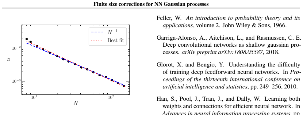
The central claim is stated in Eq. 18: for an ensemble of large finite single-hidden-layer networks with symmetric weight initialization, the probability density of outputs at a fixed input is $p_y(y) \simeq \mathcal{N}(y;0,\sigma^2)\bigl[1 - \frac{c_4(x)}{N}(3 - 6(y/\sigma)^2 + (y/\sigma)^4)\bigr]$. The skew term that would appear at order $N^{-1/2}$ vanishes because the symmetric initialization forces $c_3=0$, so the leading deviation from Gaussianity is the fourth-Hermite term at order $1/N$. The paper verifies this against ensembles of up to $10^8$ networks with ReLU activations, obtaining good agreement and measuring the perturbation amplitude to scale roughly as $N^{-1.07}$ rather than the predicted $N^{-1}$. This is an asymptotic Edgeworth expansion, so for fixed order the correction decreases as $N\to\infty$, while the full series does not converge.

Load-bearing premise

The paper derives the output density at a single input but assumes, without proof, that the joint distribution of outputs at multiple inputs is a multivariate Edgeworth expansion, and the Gaussian process picture as a distribution over functions depends on that joint behavior.

Editorial extensions

If this is right

For symmetric initializations, the output distribution of a single-hidden-layer network is never exactly Gaussian at finite width; the deviation is $O(1/N)$ and explicitly given by the fourth Hermite polynomial.
The infinite-width Gaussian process description of such networks is accurate only up to corrections of order $1/N$, with higher-order terms decaying as $N^{-n/2+1}$.
The size of the correction depends on the input through $c_4(x)$, so some inputs are more Gaussian than others at the same width.
If the $1/N$ perturbation shrinks under gradient descent, the Gaussian process and neural tangent kernel descriptions remain valid throughout training; if it grows, there may be a point where they break down.

Reading between the lines

Editorial extensions of the paper, not claims the author makes directly.

An immediate, testable consequence of the paper's own single-input result is that the joint distribution at several inputs should show $O(1/N)$ fourth-order cross-cumulants whose coefficients are products and sums of the same $c_4(x_i)$; measuring those would test the unproven multivariate step.
Because the renormalization-group argument only uses finite variance and symmetry of the weight distribution, the same leading $H_4$ structure should appear for other activations and other symmetric initializations, with only $c_4(x)$ changing.
The input-dependent $c_4(x)$ suggests that the finite-width correction acts like a small non-Gaussian field over input space, which could matter for uncertainty estimates and Bayesian model comparison even when predictions are accurate.
Tracking $c_4$ through training would turn the paper's qualitative question into a quantitative one: a measurement of whether the perturbation amplitude grows, shrinks, or stays fixed would determine whether the infinite-width limit is an attractor for training dynamics.

Share X Bluesky LinkedIn Reddit HN

Signed reviews

No signed human review yet.

Editorial analysis

A structured set of objections, weighed in public.

Desk editor's note, referee report, and a circularity audit.

Desk Editor's Note

read the letter

Joe — quick read of Antognini 1908.10030. The useful core: for a single hidden layer at init, symmetric weights, the output marginal is Gaussian plus an O(1/N) fourth-Hermite correction, and the paper shows this via a clean RG argument that recovers the classical Edgeworth expansion. That is a nice, explicit finite-width result and worth having. The RG eigenvalues are correct, Eq. 17/18 are standard, and the paper says so honestly. Credit where due: no overclaiming of novelty, the derivation is readable, and the asymptotic statement is properly qualified.

Where it gets soft. First, the abstract and Section 4 frame this as a correction to a neural network Gaussian process, i.e. a distribution over functions. The derivation only gives the one-point marginal. Footnote 3 punts on the joint distribution, but the joint is what defines a Gaussian process. Without it, the function-space conclusion is unsupported. Cross-input cumulants could enter at the same 1/N order, so this is not a minor gap in exposition; it is the difference between a marginal finite-width statement and an NNGP statement. Second, the empirics are weaker than the derivation. In section 3.1, c4 is fitted from the same CDF it is then compared to; section 3.2 fits alpha separately per width and also fits the exponent, reporting N^-1.07 rather than testing N^-1. No error bars anywhere, and only one architecture/initializer/input x=1. These are addressable, but they mean the experiments don't independently confirm the theory; they just show consistency with a fitted amplitude.

Overall: the marginal result is likely correct, the process-level claim is not established, and the experiments overstate. The paper deserves a serious referee — it is clearly written and the asymptotic structure is worth checking — but the right verdict is conditional, with the condition being joint behavior, not the one-point formula. If you cite it, cite it for the marginal Edgeworth correction, not for a rigorous NNGP finite-width theory.

Referee Report

4 major / 4 minor

Summary. The paper derives a finite-width correction to the Gaussian-process limit of a single-hidden-layer neural network at initialization. Using a renormalization-group argument for the single-input marginal distribution of the output y = Σ_i v_i f(u_i x), it obtains an Edgeworth expansion whose leading term for symmetric weight distributions is a fourth-Hermite perturbation of size c4(x)/N (Eqs. 16–18). It then reports empirical support: a comparison of empirical and predicted CDF differences at N = 128 (Sec. 3.1) and a power-law fit α ∝ N^{−1.07} (Sec. 3.2), and discusses consequences for when the NNGP framework remains valid during training.

Significance. The paper has a clear strength: the renormalization-group derivation transparently yields the scaling N^{1−n/2} for the Edgeworth corrections, and the predicted 1/N scaling of the leading non-Gaussianity is falsifiable. The observation that the Gaussian covariance is width-independent is also useful context. However, the process-level NNGP interpretation is not established: footnote 3 concedes that the multivariate Edgeworth expansion is not shown, and the numerical validation fits rather than predicts the only amplitude c4. If the paper is read as a claim about single-input marginals, it is a modest but plausible contribution; if it is read as a claim about Gaussian-process corrections, the current evidence is incomplete.

major comments (4)

[2.4, Eq. (11)] The displayed linearized eigen-equation is not the correct linearization of the renormalization operator R. For the fixed-point characteristic function g(k) = p*~(k), linearizing R gives λ_n φ~_n(k) = 2 g(k/√2) φ~_n(k/√2), and substituting φ~_n(k) = (ik)^n g(k) yields λ_n = 2^{1−n/2}. As written, Eq. (11) has an incorrect prefactor (1/(λ_n σ))√(2/π) and an exponential e^{−k²/(4σ)} that is inconsistent with the Gaussian fixed point of Eq. (9); a reader cannot reproduce Eq. (14) from the displayed equation. Please correct the equation and clarify whether σ denotes the standard deviation or the variance.
[2.4, footnote 3; Sec. 4] The paper repeatedly frames Eq. (17) as an Edgeworth expansion of a stochastic process, for instance by calling it 'the expansion of a stochastic process rather than a probability distribution.' But Eq. (17) is a statement about the marginal density of the output at one fixed input x. A stochastic process is determined by all finite-dimensional joint distributions, and footnote 3 explicitly says that the multivariate Edgeworth expansion for two or more inputs is expected but not shown. Cross-input joint cumulants could in principle enter at the same O(1/N) order as the marginal H4 term, so the process-level conclusions in Sec. 4 are not supported by the derivation or by the experiments, which evaluate only a single input. This gap is load-bearing for the NNGP framing; the authors should either prove or test the multivariate extension, or restrict their claims to single-input marginals.
[3.1, Eq. (19)] The constant c4 ≈ 9.405 is fitted from the same empirical CDF that is then compared with the predicted CDF in Fig. 1. Consequently the 'excellent agreement' in Fig. 1 is partly by construction: it validates the functional form but not the amplitude of the correction. To make the confirmation non-circular, the authors should either compute c4 from the weight distribution and moments, or fit c4 on one subset of the ensemble and compare with an independent subset. Without this, Sec. 3.1 does not provide independent evidence for Eq. (18).
[3.2, Eq. (20)] The scaling test fits α separately for each N and then fits a power law α ∝ N^{−1.07}, but no error bars or confidence intervals are reported, and the fitting procedure is not specified. Moreover, under Glorot initialization the input and output weight variances change as N varies, so c4(x) may itself depend on N; the observed exponent is therefore not a direct test of the N^{−1} prediction of Eq. (18) unless c4 is shown to be N-independent or its N-dependence is accounted for. Please provide uncertainty estimates and, if possible, a direct prediction of α(N) for the exact initialization used.

minor comments (4)

[2.3, Eq. (9)] The notation for σ is inconsistent: the text calls σ the standard deviation, but Eq. (9) writes the Gaussian Fourier transform with e^{−k²/(2σ²)}, which is not the characteristic function of N(0,σ²) under the usual convention. Please reconcile the notation and the exponential factors.
[3.2] The authors note that the small-N behavior is 'slightly steeper' than N^{−1}, but there is no discussion of where the asymptotic Edgeworth expansion is expected to break down. Reporting the residuals or a goodness-of-fit measure would help the reader assess whether the deviations are consistent with finite-N corrections.
[3.2, Eq. (20)] The text does not specify how α is fitted to each empirical CDF difference, for example whether the fit is by least squares on a grid of y values and over what range of y. This information is needed for reproducibility.
[1] Minor typographical issues include 'Tensorﬂow' with a ligature in the references; the manuscript would benefit from a final proofreading pass.

Circularity Check

1 steps flagged · score 2.0 of 10

One fitted amplitude is labeled a prediction; the central 1/N scaling is independently derived and not circular.

fitted input called prediction [Section 3.1, Eq. 19 and Fig. 1]
"We compare the empirical CDF with the predicted CDF in Fig. 1 and find excellent agreement. From this empirical CDF we measure c4≈ 9.405."

The 'predicted CDF' in Eq. 19 uses c4 as its amplitude, and c4 is measured from the very same empirical CDF that the prediction is compared against. Therefore the amplitude of the non-Gaussian correction is fitted, not independently predicted; the agreement in Fig. 1 is partially enforced by construction. What remains independently tested is only the functional shape (third Hermite polynomial times a Gaussian), not the overall size of the effect.

full rationale

The paper's core derivation in Section 2 is self-contained and non-circular: the renormalization-group fixed point is the Gaussian (Eq. 8-9), the eigenfunctions are Hermite polynomials (Eqs. 12-13), and the eigenvalues give λ_n^{log2 N} = N^{1-n/2} (Eq. 15), so the leading correction is indeed N^{-1} H4. This functional form and scaling are derived from the i.i.d. sum structure of the output, not assumed from the simulations. The N^{-1} scaling is then tested in Section 3.2 by fitting α separately for each N and inspecting its N-dependence, which is a genuine empirical check of the derived exponent. The only fitted-input concern is the amplitude c4: Section 3.1 measures c4 from the same CDF that is later called 'predicted.' This is a one-parameter shape check rather than a full prediction, and it does not affect the load-bearing N^{-1} scaling claim, so it warrants a low score rather than a high one. I also note the limitation explicitly acknowledged in footnote 3: the multivariate Edgeworth joint distribution expected for multiple inputs is not shown. This is missing support for the paper's broader 'stochastic process' framing, but it is not a circular step because it is openly identified as unproved rather than covertly assumed. The marginal Edgeworth result itself remains independently derived, so the overall circularity score is 2.

Assumptions & free parameters 3 free parameters · 4 assumptions · 0 invented entities

The only fitted free parameters are the amplitudes c4 and alpha and the fitted power-law exponent. No new physical entities are introduced. The main axioms are standard Edgeworth theory plus the i.i.d.-at-initialization and symmetric-weight assumptions specific to the setup; the multivariate Edgeworth step is an asserted extension.

free parameters (3)

c4(x) = approximately 9.405 at N=128, x=1, ReLU, Glorot uniform
Amplitude of the fourth-Hermite correction in Eq. 18; measured from the empirical CDF in section 3.1 rather than derived from the weight and activation moments.
alpha(N) = best-fit per width; scaling fit alpha proportional to N^{-1.07}
Amplitude of the CDF difference in Eq. 20, fitted separately for each N in section 3.2 to test the predicted N^{-1} scaling.
power-law exponent = -1.07
Best-fit exponent for the alpha versus N data in Fig. 2; close to but not equal to the theoretical -1.

assumptions (4)

standard math Edgeworth expansion applies to the sum of i.i.d. finite-variance random variables.
The RG fixed point in section 2.3 is the Gaussian, and the eigenvalues and eigenfunctions in section 2.4 reproduce the standard expansion; Feller 1966 and Hansen 2006 are cited.
domain assumption At initialization the summands v_i f(u_i x) are independent and identically distributed across hidden units.
Stated in section 2: 'Since the samples u_i are independent, the h_i are independent as well.' This holds for random i.i.d. weights and fixed input, but is special to initialization and single-hidden-layer networks.
domain assumption The weight distributions are symmetric, making the output summand distribution symmetric so the third Hermite term vanishes.
Section 2: 'it is generally the case that the probability distributions used to initialize NNs are symmetric and so have zero skew.' Holds for Glorot uniform but not for all initializers, as orthogonal initialization is excluded in footnote 1.
ad hoc to paper The joint distribution over multiple inputs is a multivariate Edgeworth expansion.
Footnote 3 expects this but does not derive it; the paper's conclusions about Gaussian process validity as a function-space model implicitly rely on it.

how reviews work

0 comments

Cite this review

Pith. "Pith review of Finite size corrections for neural network Gaussian processes." pith.science (2026). https://pith.science/paper/6SXCP6W3

@misc{pith2026190810030,
  author       = {Pith},
  title        = {Pith review of: Finite size corrections for neural network Gaussian processes},
  year         = {2026},
  howpublished = {\url{https://pith.science/paper/6SXCP6W3}},
  note         = {Machine review of arXiv:1908.10030}
}

read the original abstract

There has been a recent surge of interest in modeling neural networks (NNs) as Gaussian processes. In the limit of a NN of infinite width the NN becomes equivalent to a Gaussian process. Here we demonstrate that for an ensemble of large, finite, fully connected networks with a single hidden layer the distribution of outputs at initialization is well described by a Gaussian perturbed by the fourth Hermite polynomial for weights drawn from a symmetric distribution. We show that the scale of the perturbation is inversely proportional to the number of units in the NN and that higher order terms decay more rapidly, thereby recovering the Edgeworth expansion. We conclude by observing that understanding how this perturbation changes under training would reveal the regimes in which the Gaussian process framework is valid to model NN behavior.

Figures

Figures reproduced from arXiv: 1908.10030 by the authors.

**Figure 1.** and find excellent agreement. From this empirical CDF we measure c4 ≈ 9.405. 3.2. The magnitude of the perturbation and N From Eq. 18 we expect the magnitude of the deviation from a Gaussian to scale inversely with the number of hidden units, N. To test this prediction we generate a set of ensembles of randomly initialized NNs for a range of N. We vary N between 8 and 148 and for each N we use an ensemble of 107 NN… view at source ↗

**Figure 2.** The scaling of the perturbation of the distribution from a Gaussian with the number of hidden units. Each point is the best fit for α of the difference between the empirical CDF with the CDF of the third Hermite polynomial times a Gaussian (see Eq. 20). The predicted N −1 scaling is shown with the dashed blue line and the best fit scaling N −1.07 is shown with the dotted red line. the trajectories of NNs of finite s… view at source ↗

Discussion (0). Continue with ORCID to comment.

Reference graph

Works this paper leans on

12 extracted references · 3 canonical work pages

[8]

Finite size corrections for NN Gaussian processes Matthews, A. G. d. G., Rowland, M., Hron, J., Turner, R. E., and Ghahramani, Z. Gaussian process behaviour in wide deep neural networks. arXiv preprint arXiv:1804.11271,

arXiv
[9]

Paszke, A., Gross, S., Chintala, S., Chanan, G., Yang, E., DeVito, Z., Lin, Z., Desmaison, A., Antiga, L., and Lerer, A

URL https: //openreview.net/forum?id=B1g30j0qF7. Paszke, A., Gross, S., Chintala, S., Chanan, G., Yang, E., DeVito, Z., Lin, Z., Desmaison, A., Antiga, L., and Lerer, A. Automatic differentiation in pytorch. In NIPS 2017 Autodiff Workshop ,

work page 2017
[11]

and Le, Q

Tan, M. and Le, Q. V . Efﬁcientnet: Rethinking model scaling for convolutional neural networks. arXiv preprint arXiv:1905.11946,

arXiv 1905
[12]

Williams, C. K. Computing with inﬁnite networks. In Advances in neural information processing systems, pp. 295–301, 1997

work page 1997
[1966]

Garriga-Alonso, A., Aitchison, L., and Rasmussen, C. E. Deep convolutional networks as shallow gaussian pro- cesses. arXiv preprint arXiv:1808.05587,

arXiv
[1995]

Lee, J., Bahri, Y ., Novak, R., Schoenholz, S

doi: 10.1086/175420. Lee, J., Bahri, Y ., Novak, R., Schoenholz, S. S., Penning- ton, J., and Sohl-Dickstein, J. Deep neural networks as gaussian processes. arXiv preprint arXiv:1711.00165 ,

arXiv
[1999]

S., Hu, W., Li, Z., Salakhutdinov, R., and Ruosong, W

Arora, S., Du, S. S., Hu, W., Li, Z., Salakhutdinov, R., and Ruosong, W. On exact computation with an inﬁnitely wide neural net. arXiv preprint arXiv:1904:11955,

work page 1904
[2006]

Hinton, G., Vinyals, O., and Dean, J

URL http: //web.math.ku.dk/˜erhansen/bootstrap_ 05/doku/noter/Edgeworth_24_01.pdf. Hinton, G., Vinyals, O., and Dean, J. Distilling the knowledge in a neural network. arXiv preprint arXiv:1503.02531,

arXiv

Show all 12 references

[2015]

Searching for mobilenetv3

Howard, A., Sandler, M., Chu, G., Chen, L.-C., Chen, B., Tan, M., Wang, W., Zhu, Y ., Pang, R., Vasudevan, V ., et al. Searching for mobilenetv3. arXiv preprint arXiv:1905.02244,

1905 arXiv
[2017]

S., Bahri, Y ., Sohl- Dickstein, J., and Pennington, J

Lee, J., Xiao, L., Schoenholz, S. S., Bahri, Y ., Sohl- Dickstein, J., and Pennington, J. Wide neural networks of any depth evolve as linear models under gradient descent. arXiv preprint arXiv:1902.06720,

1902 arXiv
[2018]

M., McClelland, J

Saxe, A. M., McClelland, J. L., and Ganguli, S. Exact solutions to the nonlinear dynamics of learning in deep linear neural networks. arXiv preprint arXiv:1312.6120,

arXiv
[2019]

G., Zhu, M., Chen, B., Kalenichenko, D., Wang, W., Weyand, T., Andreetto, M., and Adam, H

Howard, A. G., Zhu, M., Chen, B., Kalenichenko, D., Wang, W., Weyand, T., Andreetto, M., and Adam, H. Mobilenets: Efﬁcient convolutional neural networks for mobile vision applications. arXiv preprint arXiv:1704.04861,

arXiv

Pith tools

Reviewed August 14, 2026 · model on record in the stance chip above.

[1] [8]

Finite size corrections for NN Gaussian processes Matthews, A. G. d. G., Rowland, M., Hron, J., Turner, R. E., and Ghahramani, Z. Gaussian process behaviour in wide deep neural networks. arXiv preprint arXiv:1804.11271,

arXiv

[2] [9]

Paszke, A., Gross, S., Chintala, S., Chanan, G., Yang, E., DeVito, Z., Lin, Z., Desmaison, A., Antiga, L., and Lerer, A

URL https: //openreview.net/forum?id=B1g30j0qF7. Paszke, A., Gross, S., Chintala, S., Chanan, G., Yang, E., DeVito, Z., Lin, Z., Desmaison, A., Antiga, L., and Lerer, A. Automatic differentiation in pytorch. In NIPS 2017 Autodiff Workshop ,

work page 2017

[3] [11]

and Le, Q

Tan, M. and Le, Q. V . Efﬁcientnet: Rethinking model scaling for convolutional neural networks. arXiv preprint arXiv:1905.11946,

arXiv 1905

[4] [12]

Williams, C. K. Computing with inﬁnite networks. In Advances in neural information processing systems, pp. 295–301, 1997

work page 1997

[5] [1966]

Garriga-Alonso, A., Aitchison, L., and Rasmussen, C. E. Deep convolutional networks as shallow gaussian pro- cesses. arXiv preprint arXiv:1808.05587,

arXiv

[6] [1995]

Lee, J., Bahri, Y ., Novak, R., Schoenholz, S

doi: 10.1086/175420. Lee, J., Bahri, Y ., Novak, R., Schoenholz, S. S., Penning- ton, J., and Sohl-Dickstein, J. Deep neural networks as gaussian processes. arXiv preprint arXiv:1711.00165 ,

arXiv

[7] [1999]

S., Hu, W., Li, Z., Salakhutdinov, R., and Ruosong, W

Arora, S., Du, S. S., Hu, W., Li, Z., Salakhutdinov, R., and Ruosong, W. On exact computation with an inﬁnitely wide neural net. arXiv preprint arXiv:1904:11955,

work page 1904

[8] [2006]

Hinton, G., Vinyals, O., and Dean, J

URL http: //web.math.ku.dk/˜erhansen/bootstrap_ 05/doku/noter/Edgeworth_24_01.pdf. Hinton, G., Vinyals, O., and Dean, J. Distilling the knowledge in a neural network. arXiv preprint arXiv:1503.02531,

arXiv