REVIEW 3 major objections 4 minor 34 references
Speedup in Classical Simulation of Gaussian Boson Sampling
T0 review · 3 major / 4 minor · reviewed 2026-08-14 · deepseek-v4-flash
Pith's one-line read Classical simulation of Gaussian boson sampling reaches 30 photons by splitting Hafnians into smaller pieces.
desk verdict A genuinely faster fixed-n GBS sampler based on a new Hafnian/permanent decomposition, but the full-distribution sampler has an unquantified truncation that in one of the paper's own examples discards half the distribution. read the letter →
The pith
A machine-rendered reading of the paper's core claim, the machinery that carries it, and where it could break.
The reading
What carries the argument
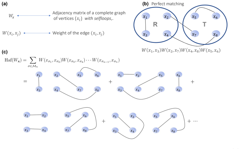
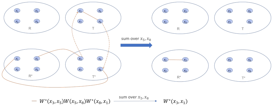
The load-bearing object is the Hafnian $\mathrm{Haf}(V)$, a matrix function like the permanent but summing over perfect matchings, which enters through the GBS output probability $p(s)=\frac{\tanh^n r}{s_1!\cdots s_m!\cosh^m r}|\mathrm{Haf}(W_s)|^2$. The paper views $W_x$ with entries $W(x_i,x_j)$ as the adjacency matrix of a complete graph with self-loops, so each matching is a collection of edges. The mechanism that carries the speedup is the summation-path rule: because $W=UU^T$ gives $\sum_i W(i,j)W^*(i,j')=\delta_{j,j'}$, a chain of unresolved internal modes in the expansion of $|\mathrm{Haf}(W_x)|^2$ contracts to a single edge, and the remaining expression collapses into a sum of products of sub-Hafnians and permanents (Theorem 1). That decomposition lets each conditional marginal be evaluated in $O(\mathrm{poly}(n)2^{8n/3})$ time, or $O(\mathrm{poly}(n)2^{5n/2})$ time if intermediate sub-Hafnians are stored in $O(m2^n)$ memory.
What would settle it
Compute the exact tail probability $T=\sum_{n>N}P_n$ for a claimed operating point (for instance $m=n^2$ with the squeezing parameters used in the 18- and 20-photon runs); if $T$ is larger than the statistical uncertainty of the benchmark, the empirical output distribution must differ measurably from exact GBS, settling the approximation question. A direct check would be to run the algorithm and brute-force sampling side by side at a feasible size, such as $n=6$ or $8$, and compare large sample sets with a chi-square statistic.
Extended reading notes
Core claim
The paper's central claim is that, for GBS with the same squeezing parameter in every input mode, sampling an output configuration $s=(s_1,\dots,s_m)$ does not require evaluating an $n\times n$ Hafnian for every configuration. The output probability factors as $p(s)=P_n p_n(s)$, where $P_n$ has a closed negative-binomial form and the conditional distribution $p_n(s)$ is independent of the squeezing parameter. By moving to an ordered list $x=(x_1,\dots,x_n)$ of photon positions, the authors express each conditional probability $q_n(x_k\mid x_1,\dots,x_{k-1})$ as a sum over pairs of perfect matchings. Using the unitarity of the interferometer matrix $W=UU^T$, internal summations over unresolved modes collapse to delta functions, and the sum reorganizes (Theorem 1) into a combination of Hafnians and permanents of submatrices, which lowers the exponent in the running time. The resulting sampling algorithm has the stated time and space bounds, simplifies to a 0-or-1 permanent in the collision-free regime, and is checked against brute-force sampling at small sizes before being extrapolated to 18, 20, and 30 photons.
Load-bearing premise
The load-bearing premise is that the photon-number distribution can be cut off at $N=c n_{\mathrm{most}}$ and renormalized without changing the sampled distribution; if the tail above $N$ is not negligible in the regimes claimed, the algorithm samples from a distribution that is not the true GBS distribution.
Editorial extensions
If this is right
- A 30-photon Gaussian boson sampling experiment could be classically sampled in about a day on a large supercomputer, so a GBS supremacy demonstration would need more than 30 photons to beat the classical benchmark.
- The exponential-space variant bounds the full photon-number-resolving simulation, including collision events, by $O(\mathrm{poly}(n)2^{5n/2})$ time.
- In the collision-free regime, where threshold detection is equivalent to photon counting, the reported limits improve on threshold-detector GBS simulation at the same sizes.
- Because $p_n(s)$ is independent of the squeezing parameter, the second stage of the algorithm applies to a whole family of GBS settings, with only the photon-number selection depending on $r$.
Reading between the lines
- The photon-number truncation at $N=c n_{\mathrm{most}}$ is renormalized without a total-variation bound; if the tail above $N$ is non-negligible, the stated 18/20/30-photon numbers describe an approximate sampler rather than exact GBS simulation.
- The same splitting technique is a general recipe for Hafnian-based marginal probabilities and should transfer to other GBS variants, such as scattershot boson sampling, threshold detection, or lossy networks, where the same unitarity contraction applies.
- A tighter analysis of the truncated tail, or a faster Hafnian subroutine plugged into Theorem 1, could move the practical simulation limit in either direction, so the supremacy threshold is not a fixed physical constant.
Signed reviews
Editorial analysis
A structured set of objections, weighed in public.
Referee Report
Summary. The paper proposes a two-step classical simulation algorithm for Gaussian boson sampling (GBS) with identical single-mode squeezed input states. In the first step, the total photon number n is sampled from the (truncated) negative-binomial distribution P_n; in the second step, a photon-mode assignment is sampled from the conditional distribution p_n(s) using a Hafnian-permanent decomposition of the marginal probabilities. The authors claim time complexity O(m sinh^2 r + poly(n)2^{8n/3}) with polynomial space and O(m sinh^2 r + poly(n)2^{5n/2}) with O(m2^n) space, and report numerical simulations of 18 photons on a laptop, 20 on a 256-core workstation, and an estimated 30 on Sunway TaihuLight. They interpret these numbers as evidence that the photon-number threshold for quantum computational supremacy with GBS is lower than for standard boson sampling.
Significance. If the algorithm is correct and the error analysis supports the practical benchmarks, this is a valuable contribution to the classical-simulation side of the quantum-supremacy debate: it gives explicit complexity exponents for GBS, provides an open-source implementation, and compares favorably with threshold-detector GBS simulations. The paper's strengths include the concrete parametric complexity derivations in Appendices C and D, the independent numerical consistency check for n=4 in Figure 6, and the de facto benchmark against brute-force sampling. However, the central claim about simulating the full GBS output distribution depends on an unquantified truncation step in Section 3.1 and on a theorem whose proof is only sketched; these points materially affect the 18/20/30-photon claims.
major comments (3)
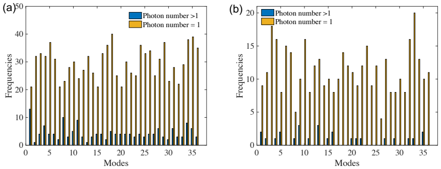
- [Section 3.1, Eq. (14), Fig. 7(b)] The truncation of the photon-number distribution is not a negligible approximation and, as stated, contradicts the paper's own numerical validation. For the parameters of Fig. 7(b), m=36 and r=0.2, we have n_most = 2 floor((m/2-1) sinh^2 r) = 2 floor(17 * 0.0405) = 0, so with N = 50 n_most the truncated support is {0}; after renormalization, Step 1 samples n=0 with probability 1, yet Fig. 7(b) reports nonzero frequencies for photon number =1 and >1. Direct evaluation of Eq. (14) gives P_0 ≈ 0.49, so the omitted tail has probability about 0.51. The manuscript must either provide a total-variation bound for the truncated sampler or explicitly restrict the claims to parameter regimes where the tail is controlled; if the benchmarks are for fixed-n conditional sampling, that needs to be stated, because then the advertised full-GBS sampler is not the implemented procedure.
- [Abstract and Section 3.5, algorithm complexity] The stated complexity O(m sinh^2 r + poly(n)2^{8n/3}) is a bound for the conditional second step at a fixed n. When Step 1 samples n from the truncated distribution, the support extends up to N = c n_most, and the second-step cost grows exponentially in the sampled n. The paper does not bound the total cost of the two-step sampler, nor the expected cost over P_n, nor the error incurred by the cutoff. Without such a bound, the advertised complexity does not describe the full GBS sampler in the form that produced the numerical benchmarks; the complexity claim should be restated as applying to conditional fixed-n sampling, with a separate analysis for the full sampler.
- [Section 3.4, Theorem 1; Appendix G; Figures 6 and 7] The correctness of the sampling algorithm rests on Theorem 1, but the proof in Appendix G is a sketch in which the counting argument for the factor F(k,mu,j1,j2) in Appendix H is asserted rather than fully derived, and no independent verification of the theorem is supplied for n>4. Figure 6 validates the full output distribution only for n=4 and m=16; Figure 7 checks only single-mode occupation frequencies, not the joint distribution. The runtime benchmarks for n=18 and n=20 therefore do not by themselves establish that the implemented sampler is drawing from the claimed distribution. A complete proof of Theorem 1, or a machine-checked verification, together with a distribution-level statistical test for a non-trivial n (for example n=8 or n=10), would be needed to support the practical claims.
minor comments (4)
- [Throughout] There are several typographical errors: 'constrcuted' in Section 2.3, 'complele' in Section 3.4.1, 'our our algorithm' in Section 3.5, 'Hafnain' in the title of Appendix F, and 'theorical' in the caption of Figure 6.
- [Section 3.5, Figure 6] The caption of Figure 6 mentions three curves (blue, green, yellow) but the text describes only two comparisons; please make the correspondence between panels and curves explicit.
- [Algorithm 2, line 10] The notation ([k]\s over mu) and the set-valued use of s are not defined before the pseudocode; a brief definition of the set notation used in Algorithm 2 would improve readability.
- [Abstract and Table 1] The phrase 'establish a lower bound for achieving quantum computational supremacy' is imprecise: the paper gives an upper bound on classical simulation cost, from which one infers a lower bound on the photon number needed for a quantum advantage claim. Rephrasing would avoid confusion.
Circularity Check
No significant circularity: the GBS sampling algorithm is derived from Hafnian, permanent, and unitarity identities, and the practical photon-number limits are runtime extrapolations rather than fitted inputs.
full rationale
The paper's central derivation is self-contained: it starts from the standard GBS output probability p(s) expressed through Hafnians (Eq. 9), derives the conditional distribution p_n(s) (Eq. 15), changes to the first-quantized position basis (Eqs. 16-20), and then decomposes each marginal probability by summing over perfect matchings and applying the unitarity relation sum_i W(i,j)W*(i,j') = delta(j,j') (Rule 3). The resulting Theorem 1 and the complexity bounds O(poly(n)2^{8n/3}) and O(poly(n)2^{5n/2}) follow from counting these matching terms and from the cited Hafnian complexity of Björklund et al., not from any fitted parameter or from the paper's own conclusions. The numerical claims for 18, 20, and 30 photons are extrapolations from measured runtimes on actual hardware against the operation count of the algorithm; they are not used as inputs to define the algorithm. The paper does cite its own source code (Ref. [32]), but that citation is not load-bearing for any mathematical claim. The truncation of the photon-number distribution at N = c n_most is an approximation without a proven total-variation bound, and the Fig. 7(b) parameters may even make n_most = 0 while nonzero photon numbers are reported, but this is a correctness or consistency concern, not circularity. No step in the derivation is equivalent by construction to its own input, and no prediction is a renamed fit. Therefore the circularity score is 0.
Assumptions & free parameters
free parameters (1)
- truncation cutoff factor c =
50 (set for numerics)
assumptions (4)
- domain assumption Input states are single-mode squeezed states with identical squeezing parameter r in every mode.
- ad hoc to paper The tail of the photon-number distribution beyond N=c n_most is negligible, so renormalizing the truncated distribution yields a sample close to the exact GBS distribution.
- standard math The unitarity relation sum_i W(i,j)W*(i,j') = delta(j,j') permits summation paths to be replaced by single edges (Rule 3).
- standard math The combinatorial identity of Eq. (60) (from Graham et al.) is used to simplify the factor F(k,mu,j1,j2).
Cite this review
Pith. "Pith review of Speedup in Classical Simulation of Gaussian Boson Sampling." pith.science (2026). https://pith.science/paper/JQCXWM64
@misc{pith2026190810070,
  author       = {Pith},
  title        = {Pith review of: Speedup in Classical Simulation of Gaussian Boson Sampling},
  year         = {2026},
  howpublished = {\url{https://pith.science/paper/JQCXWM64}},
  note         = {Machine review of arXiv:1908.10070}
}
read the original abstract
Gaussian boson sampling is a promising model for demonstrating quantum computational supremacy, which eases the experimental challenge of the standard boson-sampling proposal. Here by analyzing the computational costs of classical simulation of Gaussian boson sampling,we establish a lower bound for achieving quantum computational supremacy for a class of Gaussian boson-sampling problems, where squeezed states are injected into every input mode. Specifically, we propose a method for simplifying the brute-force calculations for the transition probabilities in Gaussian boson sampling, leading to a significant reduction of the simulation costs. Particularly, our numerical results indicate that we can simulate 18 photons Gaussian boson sampling at the output subspace on a normal laptop, 20 photons on a commercial workstation with 256 cores, and suggest about 30 photons for supercomputers. These numbers are significantly smaller than those in standard boson sampling, suggesting Gaussian boson sampling may be more feasible for demonstrating quantum computational supremacy.
Figures

Figures from the paper (6 more)




Reference graph
Works this paper leans on
-
[1]
The computational complexity of linear optics
Scott Aaronson and Alex Arkhipov. The computational complexity of linear optics. In Proceedings of the forty-third annual ACM symposium on Theory of computing , pages 333–342. ACM, 2011
work page 2011
-
[2]
Complexity-theoretic foundations of quantum supremacy experiments
Scott Aaronson and Lijie Chen. Complexity-theoretic foundations of quantum supremacy experiments. In LIPIcs-Leibniz International Proceedings in Informat- ics, volume 79. Schloss Dagstuhl-Leibniz-Zentrum fuer Informatik, 2017
work page 2017
-
[3]
Using Gaussian Boson Sampling to Find Dense Subgraphs
Juan Miguel Arrazola and Thomas R Bromley. Using gaussian boson sampling to find dense subgraphs. arXiv preprint arXiv:1803.10730 , 2018
work page Pith review arXiv 2018
-
[4]
Molecular Docking with Gaussian Boson Sampling
Leonardo Banchi, Mark Fingerhuth, Tomas Babej, Juan Miguel Arrazola, et al. Molecular docking with gaussian boson sampling. arXiv preprint arXiv:1902.00462 , 2019
work page Pith review arXiv 1902
-
[5]
A faster hafnian formula for complex matrices and its benchmarking on the titan supercomputer
Andreas Bj¨ orklund, Brajesh Gupt, and Nicol´ as Quesada. A faster hafnian formula for complex matrices and its benchmarking on the titan supercomputer. arXiv preprint arXiv:1805.12498, 2018
arXiv 2018
-
[6]
Character- izing quantum supremacy in near-term devices
Sergio Boixo, Sergei V Isakov, Vadim N Smelyanskiy, Ryan Babbush, Nan Ding, Zhang Jiang, Michael J Bremner, John M Martinis, and Hartmut Neven. Character- izing quantum supremacy in near-term devices. Nature Physics, 14(6):595, 2018
work page 2018
-
[7]
Simula- tion of low-depth quantum circuits as complex undirected graphical models
Sergio Boixo, Sergei V Isakov, Vadim N Smelyanskiy, and Hartmut Neven. Simula- tion of low-depth quantum circuits as complex undirected graphical models. arXiv preprint arXiv:1712.05384, 2017
arXiv 2017
-
[8]
Gaussian boson sampling for perfect matchings of arbitrary graphs
Kamil Br´ adler, Pierre-Luc Dallaire-Demers, Patrick Rebentrost, Daiqin Su, and Christian Weedbrook. Gaussian boson sampling for perfect matchings of arbitrary graphs. arXiv preprint arXiv:1712.06729 , 2017
arXiv 2017
Show all 34 references
-
[9]
Classical simulation of commuting quantum computations implies collapse of the polynomial hierarchy
Michael J Bremner, Richard Jozsa, and Dan J Shepherd. Classical simulation of commuting quantum computations implies collapse of the polynomial hierarchy. In Proceedings of the Royal Society of London A: Mathematical, Physical and Engineer- ing Sciences, page rspa20100301. The...
2010
-
[10]
Classical simulation of intermediate-size quantum circuits
Jianxin Chen, Fang Zhang, Mingcheng Chen, Cupjin Huang, Michael Newman, and Yaoyun Shi. Classical simulation of intermediate-size quantum circuits. arXiv preprint arXiv:1805.01450, 2018
2018 arXiv
-
[11]
64-qubit quantum circuit simulation
Zhao-Yun Chen, Qi Zhou, Cheng Xue, Xia Yang, Guang-Can Guo, and Guo-Ping Guo. 64-qubit quantum circuit simulation. Science Bulletin, 2018
2018
-
[12]
The classical complexity of boson sampling
Peter Clifford and Rapha¨ el Clifford. The classical complexity of boson sampling. In Proceedings of the Twenty-Ninth Annual ACM-SIAM Symposium on Discrete Algo- rithms, pages 146–155. Society for Industrial and Applied Mathematics, 2018
2018
-
[13]
The sunway taihu- light supercomputer: system and applications
Haohuan Fu, Junfeng Liao, Jinzhe Yang, Lanning Wang, Zhenya Song, Xiaomeng Huang, Chao Yang, Wei Xue, Fangfang Liu, Fangli Qiao, et al. The sunway taihu- light supercomputer: system and applications. Science China Information Sciences , 59(7):072001, 2016
2016
-
[14]
Introductory quantum optics
Christopher Gerry, Peter Knight, and Peter L Knight. Introductory quantum optics. Cambridge university press, 2005. 15
2005
-
[15]
Concrete mathematics: a foundation for computer science
Ronald L Graham, Donald E Knuth, Oren Patashnik, and Stanley Liu. Concrete mathematics: a foundation for computer science. Computers in Physics , 3(5):106– 107, 1989
1989
-
[16]
Brajesh Gupt, Juan Miguel Arrazola, Nicols Quesada, and Thomas R. Bromley. Classical benchmarking of Gaussian Boson Sampling on the Titan supercomputer. arXiv:1810.00900, October 2018. arXiv: 1810.00900
2018 arXiv
-
[17]
Hamilton, Regina Kruse, Linda Sansoni, Sonja Barkhofen, Christine Silber- horn, and Igor Jex
Craig S. Hamilton, Regina Kruse, Linda Sansoni, Sonja Barkhofen, Christine Silber- horn, and Igor Jex. Gaussian Boson Sampling. Physical Review Letters , 119(17), October 2017
2017
-
[18]
Quantum computational supremacy
Aram W Harrow and Ashley Montanaro. Quantum computational supremacy. Na- ture, 549(7671):203, 2017
2017
-
[19]
Negative binomial regression
Joseph M Hilbe. Negative binomial regression. Cambridge University Press, 2011
2011
-
[20]
A detailed study of gaussian boson sampling
Regina Kruse, Craig S Hamilton, Linda Sansoni, Sonja Barkhofen, Christine Silber- horn, and Igor Jex. A detailed study of gaussian boson sampling. arXiv preprint arXiv:1801.07488, 2018
2018 arXiv
-
[21]
Quantum supremacy circuit simulation on sunway taihulight
Riling Li, Bujiao Wu, Mingsheng Ying, Xiaoming Sun, and Guangwen Yang. Quantum supremacy circuit simulation on sunway taihulight. arXiv preprint arXiv:1804.04797, 2018
2018 arXiv
-
[22]
Boson sampling from a gaussian state
AP Lund, A Laing, S Rahimi-Keshari, T Rudolph, Jeremy L OBrien, and TC Ralph. Boson sampling from a gaussian state. Physical review letters, 113(10):100502, 2014
2014
-
[23]
Classical boson sampling algorithms with superior performance to near-term experiments
Alex Neville, Chris Sparrow, Rapha¨ el Clifford, Eric Johnston, Patrick M Birchall, Ashley Montanaro, and Anthony Laing. Classical boson sampling algorithms with superior performance to near-term experiments. Nature Physics, 13(12):1153, 2017
2017
-
[24]
Classical simulation of photonic linear optics with lost particles
Micha l Oszmaniec and Daniel J Brod. Classical simulation of photonic linear optics with lost particles. arXiv preprint arXiv:1801.06166 , 2018
2018 arXiv
-
[25]
Breaking the 49-qubit barrier in the simulation of quantum circuits
Edwin Pednault, John A Gunnels, Giacomo Nannicini, Lior Horesh, Thomas Mager- lein, Edgar Solomonik, and Robert Wisnieff. Breaking the 49-qubit barrier in the simulation of quantum circuits. arXiv preprint arXiv:1710.05867 , 2017
-
[26]
Gaussian boson sam- pling using threshold detectors
Nicol´ as Quesada, Juan Miguel Arrazola, and Nathan Killoran. Gaussian boson sam- pling using threshold detectors. Physical Review A, 98(6):062322, 2018
2018
-
[27]
The classical complexity of gaussian boson sampling
Nicols Quesada and Juan Miguel Arrazola. The classical complexity of gaussian boson sampling. arXiv preprint arXiv:1908.08068 , 2019
1908 arXiv
-
[28]
Noise in bosonsampling and the threshold of efficient classical simulability
Valery Shchesnovich. Noise in bosonsampling and the threshold of efficient classical simulability. arXiv preprint arXiv:1902.02258 , 2019
1902 arXiv
-
[29]
Temporally unstructured quantum compu- tation
Dan Shepherd and Michael J Bremner. Temporally unstructured quantum compu- tation. In Proceedings of the Royal Society of London A: Mathematical, Physical and Engineering Sciences, volume 465, pages 1413–1439. The Royal Society, 2009
2009
-
[30]
Adaptive quantum computation, constant depth quantum circuits and arthur-merlin games
Barbara M Terhal and David P DiVincenzo. Adaptive quantum computation, constant depth quantum circuits and arthur-merlin games. arXiv preprint quant- ph/0205133, 2002
2002
-
[31]
The complexity of computing the permanent
Leslie G Valiant. The complexity of computing the permanent. Theoretical computer science, 8(2):189–201, 1979
1979
-
[32]
The source code of classical sampling algorithm for gaussian boson sampling
Bujiao Wu, Bin Cheng, Jialin Zhang, Man-Hong Yung, and Xiaoming Sun. The source code of classical sampling algorithm for gaussian boson sampling. https://github.com/GillianOoO/Classical-Simulation-of-GBS, 2018. 16 A Proof of the normalization of qn(x) Proof. By the definition o...
2018
-
[33]
Suppose M1,M 2 are two perfect matchings of ( Ra,T a′,G e,e′) and ( Rθ,Tθ′,G b,b′) repectively
For any two different vertex sets ( a, a′, e, e′) and (θ,θ′, b, b′), suppose a⁄= θ, then there exists a vertex u in a and b simultaneously (Since (θ, b) is a partition of [k]). Suppose M1,M 2 are two perfect matchings of ( Ra,T a′,G e,e′) and ( Rθ,Tθ′,G b,b′) repectively. Suppo...
-
[34]
Suppose M is a perfect matching in G. In the following we prove that there exists a quadruple ( a, a′, e, e′) and a perfect matching triple ( M1,M 2,M 3) of their repre- senting triple (Ra,T a′,G e,e′), such that (M1,M 2,M 3) construct M. As in figure ??, we partition the verte...
Reviewed August 14, 2026 · model on record in the stance chip above.
Discussion (0). Continue with ORCID to comment.