Robust Trajectory Tracking Control for Underactuated Autonomous Underwater Vehicles

Alexandros Nikou; Dimos V. Dimarogonas; Shahab Heshmati-Alamdari

REVIEW 4 major objections 5 minor 38 references

Robust Trajectory Tracking Control for Underactuated Autonomous Underwater Vehicles

T0 review · 4 major / 5 minor · reviewed 2026-08-14 · deepseek-v4-flash

Challenge this review Re-run · record.json Download PDF Read on arXiv ↗ Review JSON

Pith's one-line read Tube-based NMPC makes underactuated AUVs input-to-state stable despite currents and model error.

desk verdict Tube-based NMPC applied to underactuated AUV tracking, but a wrong yaw-rate term in the error dynamics (eq. 20) breaks the model that Theorem 1 relies on. read the letter →

arxiv 1908.10175 v2 pith:DTI2FHDC submitted 2019-08-27 cs.RO

Shahab Heshmati-alamdari , Alexandros Nikou , Dimos V. Dimarogonas This is my paper · ORCID

classification cs.RO

keywords underactuatedautonomousunderwatervehicletrajectorytrackingtube-basedmodelpredictivecontrolrobustinvariantsetinput-to-statestabilityobstacleavoidanceexternaldisturbancesfinitehorizonoptimal

verification ladder T0 review T1 audit T2 compute T3 formal

The pith

A machine-rendered reading of the paper's core claim, the machinery that carries it, and where it could break.

The reading

This paper tackles the problem of steering an underactuated autonomous underwater vehicle (actuated only in surge, heave, and yaw) along a 3D reference trajectory while respecting input limits and avoiding obstacles in a partially known, dynamic workspace. The authors propose a robust nonlinear model predictive controller in which an online optimizer plans for the nominal (disturbance-free) error dynamics, while an off-line linear feedback law keeps the real trajectory inside a hyper-tube of radius $\tilde{\rho}$ around the nominal one. The central claim is that if the finite-horizon optimal control problem is feasible at time zero, the closed-loop system is input-to-state stable with respect to currents, waves, and unmodeled dynamics, and every detected obstacle is avoided by construction. The value of the result is that robustness is achieved without solving a stochastic or min-max optimization online; the disturbance rejection is encoded in the off-line tube and the tightened constraints.

What carries the argument

The load-bearing mechanism is tube-based model predictive control built around a robust control invariant set. For the error dynamics (21), the deviation $\rho$ between the real error and the nominal error evolves as (25). A linear feedback $\kappa(e,\hat{e}) = -\sigma(e - \hat{e})$ is chosen so that the time derivative of $\Lambda(\rho) = \frac{1}{2}\|\rho\|^2$ is negative outside the ball of radius $\tilde{\rho} = \tilde{\xi}/(\sigma J - L_1 - L_2)$, where $J$ is a lower bound on the symmetrized Jacobian of $J(e,p_d)$, $L_1$ and $L_2$ are Lipschitz constants of $h$ and $\zeta$, and $\tilde{\xi}$ is the bound on the disturbance term $\xi(e,\omega)$. The nominal trajectory is generated by an FHOCP solved for the nominal error dynamics (22), with state and input constraints tightened by the tube: $\tilde{E} = E \ominus \mathcal{P}$ and $\tilde{V} = V \ominus [-\sigma \circ \mathcal{P}]$. The prediction horizon is capped by $T \le \bar{R}/(\bar{V} + \tilde{\xi})$ so that any newly detected obstacle lies within the sensing range during the horizon. The proof of the theorem follows the quasi-infinite horizon NMPC stability framework and a tube-based MPC proof with a robust control invariant set for Lipschitz nonlinear systems.

What would settle it

Compute $L_1$, $L_2$, $J$, and $\tilde{\xi}$ for a concrete AUV model over the operating envelope. If $\sigma J - L_1 - L_2 \le 0$ for any admissible $\sigma$, or if the tightened state set $E \ominus \mathcal{P}$ is empty, then the hyper-tube invariant set $\mathcal{P}$ does not exist and the ISS guarantee of Theorem 1 cannot hold. Alternatively, run the simulation with a disturbance sequence whose norm touches $\tilde{\xi}$ and check whether $\|e(t) - \hat{e}(t)\|$ ever exceeds $\tilde{\rho}$; any violation falsifies the robust invariance claim.

Watch

Extended reading notes

Core claim

The paper's central claim is Theorem 1: under feasibility of the FHOCP (31a)-(31d) at $t=0$, the control law $v = \hat{v}(\hat{e}) - \sigma(e - \hat{e})$ renders the closed-loop system input-to-state stable with respect to the disturbance vector $\omega$, for every initial condition in the nominal error set $\hat{e}(0)\in\tilde{E}$. The proof combines two facts: the nominal error dynamics are asymptotically stabilized by the receding-horizon solution, and the deviation $\rho(t) = e(t) - \hat{e}(t)$ remains inside the ball $\mathcal{P} = \{\rho: \|\rho\| \le \tilde{\rho}\}$ because the feedback law makes the Lyapunov function $\Lambda(\rho) = \frac{1}{2}\|\rho\|^2$ decrease whenever $\|\rho\|$ exceeds $\tilde{\xi}/(\sigma J - L_1 - L_2)$. Consequently, the real trajectory is the nominal trajectory inflated by a tube of radius $\tilde{\rho}$, so tightening the state and input constraint sets by that tube suffices to guarantee obstacle avoidance and input saturation despite disturbances.

Load-bearing premise

The guarantee collapses if the Lipschitz constants $L_1$, $L_2$, the Jacobian lower bound $J$, and the disturbance bound $\tilde{\xi}$ are not known finite numbers that satisfy $\sigma J - L_1 - L_2 > 0$, since the tube radius and the tightened constraint sets are built from them.

Editorial extensions

If this is right

Feasibility of the nominal FHOCP at startup is the only online condition needed: once it holds, the same controller keeps tracking and safety for all future disturbances bounded by $\bar{\omega}$.
The real trajectory never leaves the hyper-tube around the nominal one, so obstacle avoidance and input saturation reduce to an offline geometric tightening of the constraint sets, not an online robustness computation.
Because the FHOCP solves only the nominal dynamics, the computational cost of the robust controller matches that of a standard NMPC, making real-time implementation plausible.
The horizon constraint $T \le \bar{R}/(\bar{V} + \tilde{\xi})$ ensures that any obstacle entering the sensing region is seen early enough to be incorporated into the re-planned nominal trajectory, so the obstacle-avoidance guarantee covers newly detected obstacles, not just pre-known ones.

Reading between the lines

Editorial extensions of the paper, not claims the author makes directly.

The same tube construction would apply to multi-AUV scenarios if each vehicle treats the others as an additional bounded disturbance, though the required coupling bounds are not analyzed here.
An implementation would first need an identification step to compute or conservatively estimate $L_1$, $L_2$, $J$, and $\tilde{\xi}$ from the actual vehicle; the paper's guarantee is conditional on these constants satisfying the strict inequality.
There is an implicit trade-off between disturbance rejection and feasibility: increasing $\sigma$ shrinks $\tilde{\rho}$ but shrinks the tightened input set $\tilde{V}$, which may make the FHOCP infeasible for aggressive maneuvers.
The spherical-world representation means the obstacle guarantee is conservative: any convex obstacle could be handled by inflating it by the tube radius, a straightforward extension the paper does not state.

Share X Bluesky LinkedIn Reddit HN

Signed reviews

No signed human review yet.

Editorial analysis

A structured set of objections, weighed in public.

Desk editor's note, referee report, and a circularity audit.

Desk Editor's Note

read the letter

The paper applies a known tube-based NMPC framework to trajectory tracking for an underactuated AUV with obstacle avoidance. The combination is arguably new: the error model, online obstacle detection, and a sensing-range-limited horizon are not in the cited prior work. The spherical-world setup and the tightened-constraint idea are standard but fit the problem well. A simulation shows the controller avoiding two obstacles while tracking a circle, with error and input plots. That part is fine.

The trouble is the dynamics. Equation (16) defines e_o = (e_x/e_d) sinψ − (e_y/e_d) cosψ. Differentiating that using (6), the coefficient of yaw rate r is (e_x cosψ + e_y sinψ)/e_d, not e_x e_y/e_d² as written in (20) and in the third row of J(e,p_d) in (21). A direct test: e_x=1, e_y=0, ψ=0, u=w=0, r=1 gives e_o=0 and the true e_ȯ=1, while (20) gives 0. So the FHOCP in (31) is solved for a model that differs from the actual error kinematics. Theorem 1's ISS claim and the obstacle-avoidance guarantee are therefore not established for the real vehicle. This is not a minor typo; the whole tube calculation in Lemma 1 and the tightened constraints in (32) use the wrong Jacobian.

There are other soft spots of varying size. The set E is defined in (17) as a subset of R⁴ via x∈X, but (31c) uses it for the R³ error vector; that's a dimension mismatch, fixable by redefining E properly. The constants J, L₁, L₂, ξ̄ that determine the tube radius ρ̄ are asserted to exist (Remarks 1–2) but never computed or bounded, so the guarantee is not constructively instantiated. Theorem 1's proof is explicitly delegated to the authors' prior papers, and the recursive feasibility argument is omitted. The simulation has no baseline or comparison, which limits its evidential value, though that is a minor issue.

Is the central idea sound? Possibly. The tube-based machinery is well established, and the application is sensible. But the load-bearing model error means the paper, as it stands, does not deliver what it claims. I would not cite it until the error dynamics are fixed and the constants are actually instantiated.

Would I send it to peer review? Yes. The topic is relevant, the framework is standard, and the flaws are specific and fixable. A serious referee should catch the yaw-rate issue and request a corrected derivation. It deserves referee time, not desk rejection, but it needs substantial revision before it is publishable.

Referee Report

4 major / 5 minor

Summary. The paper proposes a robust nonlinear model predictive control (NMPC) scheme for an underactuated autonomous underwater vehicle (AUV) tracking a 3D trajectory in a workspace with obstacles and external disturbances. The controller combines a finite-horizon optimal control problem (FHOCP) solved for nominal error dynamics with an off-line state-feedback tube controller, aiming to keep the real trajectory in a hyper-tube around the nominal trajectory. The main theorem (Theorem 1) claims input-to-state stability of the closed loop and obstacle avoidance for all detected obstacles under the proposed feedback law. A MATLAB simulation study is included to illustrate the behavior of the controller.

Significance. If the theoretical guarantees were established, the proposed tube-based NMPC architecture would be a useful contribution to robust trajectory tracking for underactuated AUVs, particularly for the combination of input constraints, state constraints, and obstacle avoidance. The problem is well motivated and the control architecture is clearly presented. However, the main theorem is not proved in the paper, and the error dynamics used throughout the tube analysis contain a derivational error. As a result, the paper's central theoretical claims are currently unsupported. The simulation study is a useful illustration but does not substitute for a correct proof. The paper ships no machine-checked proofs or reproducible code, and the key design constants are left unspecified.

major comments (4)

[IV-A, Eq. (20)] Equation (20) does not give the correct time derivative of the orientation error defined in (16). From e_o = (e_x/e_d) sin(psi) - (e_y/e_d) cos(psi) and the kinematic equation (6), the coefficient of r in e_o-dot is (e_x cos(psi) + e_y sin(psi))/e_d, not e_x e_y/e_d^2, and the derivative also contains a term proportional to e_d-dot/e_d^2 that is omitted. A direct test is: with e_x=1, e_y=0, psi=0, u=w=0, r=1 and zero disturbances and desired velocity, (16) gives e_o=0 and the true e_o-dot equals r=1, while (20) gives 0. Since (21), (22), (25), Lemma 1, and the tightened constraints in (32) all build on this erroneous J(e,pd), the FHOCP (31) is solved for a model that is not the actual error system, so Theorem 1's ISS and obstacle-avoidance claims are not established for the real vehicle.
[IV-C, Theorem 1] The proof of Theorem 1 is not provided. The text states that the feasibility proof follows [31], [35], [36] and is omitted, and the nominal asymptotic stability is invoked via a class KL bound without proving that the FHOCP (31) with terminal set (33) delivers this property. In particular, recursive feasibility of (31) under the terminal set and tightened constraints is a load-bearing step for the claimed ISS result and must be demonstrated or precisely imported from the cited works with all hypotheses verified.
[IV-A, Eq. (17) and IV-C, Eq. (31c)] The feasible error set E is defined in (17) as a subset of R4 (since x is in X subset of R4), but the FHOCP (31c) imposes ^e(s) in E with ^e in R3. The paper does not define the projection from the state space X to the error space [ed, ez, eo], nor does it explain how the constraints on x translate to constraints on e. Consequently, the tightened constraint sets in (32) are not well-defined in the space in which the FHOCP is solved.
[IV-B, Lemma 1 and Remarks 1-2] The constants L1, L2, J, and ~xi are asserted to exist but are never computed or bounded. The tube radius ~rho = ~xi/(sigma J - L1 - L2) and the tightened sets E and V in (32) depend directly on these values; without concrete bounds or a method to compute them from the vehicle parameters and the disturbance bound ~omega, the proposed controller cannot be instantiated and the claimed robustness guarantee is not constructive.

minor comments (5)

[Abstract and VI] The abstract contains a typo ('or 3D trajectories' for 'of 3D trajectories'), and the conclusion misspells 'Vehicles' as 'Vehciles'.
[III-A] The notation for the sway velocity v and the disturbance bound ~v is confusing: in (4) ~v bounds the sway velocity, while in (13) ~V is the input bound; consider renaming one of these to avoid ambiguity. Also, the description of the current parameters delta_x, delta_y, delta_z and delta_c is unclear and should be restated.
[IV-C, Eq. (31c) and surrounding text] In (31c), 'for all delta t in [t_k, t_k+T]' should presumably read 'for all s in [t_k, t_k+T]', and (31a) writes '^u(s)' while the control input is denoted ^v elsewhere. In the sentence after (32), 'the real error states e and the real control input v satisfy the state and input constraints E, P and U' should refer to the sets E and V, not 'P and U'.
[IV-B and IV-C] The symbol P is overloaded: it denotes the error-tube set in Lemma 1, a positive definite matrix in the cost function (31a), and the terminal set F in (33) uses ||^e||_P. This overloading makes the text hard to follow; distinct notations should be used.
[V] The simulation study does not report the values of the design constants L1, L2, J, ~xi, sigma, or the resulting tube radius ~rho, making it impossible to verify that the simulated controller actually corresponds to the proposed scheme and to the condition (28).

Circularity Check

0 steps flagged · score 0.0 of 10

No circularity found: the tube-based NMPC derivation is built from explicit error dynamics and an in-text invariance lemma; the only self-citations are prior general tube-MPC results, not restatements of this paper's claims.

full rationale

The paper's central chain is: define error states (14)-(16), compute the nominal/perturbed error dynamics (18)-(21), prove Lemma 1 in the text that the feedback law (27) renders a bounded tube invariant under Lipschitz and bounded-disturbance assumptions, and then formulate FHOCP (31) over the nominal dynamics with tightened constraints (32). No parameter is fitted to data and then renamed a prediction, and no quantity in Theorem 1 is defined in terms of the theorem's conclusion. The proof of Theorem 1 delegates feasibility and nominal-stability arguments to [31], [35], [36]; [35] and [36] are prior works by the same authors, but they are general tube-based MPC results on uncertain nonlinear and multi-agent systems and do not presuppose the AUV-specific error model or obstacle-avoidance claim made here, so this is imported external support rather than a circular reduction. Concerns such as the uncomputed Lipschitz constants L1, L2, J, and xi_bar and the possible algebraic error in Eq. (20) affect the soundness or constructiveness of the guarantees, not whether the derivation is equivalent to its inputs; no circular step can be exhibited from the text.

Assumptions & free parameters 4 free parameters · 5 assumptions · 0 invented entities

The central guarantee rests on several uncomputed constants and on results imported from the authors' own prior work. No new physical entities are introduced.

free parameters (4)

Feedback gain sigma = not specified
Required to satisfy sigma > (L1+L2)/J in (28); no numerical value or tuning procedure is given, though tube invariance depends on it.
Lipschitz constants L1, L2 = not specified
Defined in (26) but never bounded or computed for the AUV error dynamics; they set the tube radius and the sigma condition.
Jacobian lower bound J = not specified
Assumed positive in Remark 1 but never quantified for the error Jacobian J(e,pd).
Disturbance bound xi_bar = not specified
Upper bound of xi(e,omega) in Remark 2 is stated to exist but not quantified; it directly sets the tube radius in Lemma 1.

assumptions (5)

domain assumption The sway velocity v is a bounded perturbation with bound v_bar, so the nominal kinematic system (3) neglects g(x,v).
Taken from [28] via ISS; the real system (6) then treats sway as a disturbance, which is load-bearing for the error model (21).
domain assumption Roll and pitch dynamics are negligible, with phi=theta=0 and p=q=0, due to metacentric restoring forces and low speed.
Used to reduce the 6-DOF model to the 4-state model (2); standard for AUVs but unvalidated here.
ad hoc to paper Finite Lipschitz constants L1, L2 and a positive lower bound J exist such that (26) and Remark 1 hold.
Stated as facts without computation; the tube invariance proof in Lemma 1 depends on them.
domain assumption The FHOCP remains feasible at every sampling time.
Used in Theorem 1; the proof is not given in this paper and is delegated to [31], [35], [36].
domain assumption Obstacles are disjoint spheres satisfying (8), so a feasible gap exists between them.
The spherical world assumption from [29] guarantees the vehicle can pass between obstacles; this underpins the state constraint set X in (11).

how reviews work

0 comments

Cite this review

Pith. "Pith review of Robust Trajectory Tracking Control for Underactuated Autonomous Underwater Vehicles." pith.science (2026). https://pith.science/paper/DTI2FHDC

@misc{pith2026190810175,
  author       = {Pith},
  title        = {Pith review of: Robust Trajectory Tracking Control for Underactuated Autonomous Underwater Vehicles},
  year         = {2026},
  howpublished = {\url{https://pith.science/paper/DTI2FHDC}},
  note         = {Machine review of arXiv:1908.10175}
}

read the original abstract

Motion control of underwater robotic vehicles is a demanding task with great challenges imposed by external disturbances, model uncertainties and constraints of the operating workspace. Thus, robust motion control is still an open issue for the underwater robotics community. In that sense, this paper addresses the tracking control problem or 3D trajectories for underactuated underwater robotic vehicles operating in a constrained workspace including obstacles. In particular, a robust Nonlinear Model Predictive Control (NMPC) scheme is presented for the case of underactuated Autonomous Underwater Vehicles (AUVs) (i.e., vehicles actuated only in surge, heave and yaw). The purpose of the controller is to steer the underactuated AUV to a desired trajectory with guaranteed input and state constraints within a partially known and dynamic environment where the knowledge of the operating workspace is constantly updated on-line via the vehicle's on-board sensors. In particular, by considering a ball that covers the volume of the system, obstacle avoidance with any of the detected obstacles is guaranteed, despite the model dynamic uncertainties and the presence of external disturbances representing ocean currents and waves. The proposed feedback control law consists of two parts: an online law which is the result of a Finite Horizon Optimal Control Problem (FHOCP) solved for the nominal dynamics; and a state feedback law which is tuned off-line and guarantees that the real trajectories remain bound in a hyper-tube centered along the nominal trajectories for all times. Finally, a simulation study verifies the performance and efficiency of the proposed approach.

Figures

Figures reproduced from arXiv: 1908.10175 by the authors.

**Figure 1.** The underactuated underwater vehicle. Blue color indicates the actuated degrees of freedom. block diagonal matrix with the matrices P1, . . . , Pn in the main diagonal; B(c, r) := {x ∈ R n : kx − ck2 ≤ r} , stands for a ball in R n with center and radius c ∈ R n, r > 0, respectively. Given sets S1, Z ⊆ R n, S2 ⊆ R m and matrix P ∈ R n×m, the Minkowski addition, the Pontryagin difference and the matrix-set multiplic… view at source ↗

**Figure 2.** Graphical illustration of the error and the sea current definitions. Notice that the v indicates the vehicle velocity in the sway direction. In [28], using Input-to-State Stability (ISS) framework, it was shown that for any vehicle described by (2) and for any bounded control input [u, r] the velocity around the sway direction v can be seen as a bounded perturbation with upper bound ||v|| ≤ v¯. Consequently, this p… view at source ↗

**Figure 3.** The hyper-tube centered along the trajectory eˆ(t) (depicted by the blue line) with radius ρe. Under the proposed control law, the real trajectory e(t) (depicted with red line) lies inside the hyper-tube for all times, i.e., kρ(t)k ≤ ρe, ∀t ∈ R≥0. renders the set: P := {ρ ∈ R n : kρk ≤ ρe} , an RCI set for the error dynamics (25), according to Definition 1, with: ρe := ξe σJ − L1 − L2 > 0. Proof : Consider the posi… view at source ↗

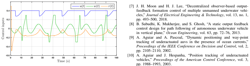
Figures from the paper (3 more)

**Figure 4.** Figure 4: Simulation setup: underactuated AUV operating in workspace including obstacles. The sensing range of the robot is indicated by a blue circle region around the robot. The desired trajectory is depicted with green dashed line which coincides with obstacles positions. The…

**Figure 5.** Figure 5: The evolution of the error over time. The four peaks in ed and ez stand for the fact that the robot is leaving the desired trajectory in order to avoid the obstacles. and r¯ = 0.5 rad s . Moreover, the capability sensing range and the horizon of the FHOCP are considere…

**Figure 6.** Figure 6: The evolution of the control input signals over time. found in the following link: https://youtu.be/jJfjnp-mw s VI. CONCLUSIONS AND FUTURE WORK This paper presents a robust trajectory tracking control for underactuated Autonomous Underwater Vehciles operating in a cons…

Discussion (0). Continue with ORCID to comment.

Reference graph

Works this paper leans on

38 extracted references · 37 canonical work pages

[31]

A Quasi-Inﬁnite Horizon Nonlinear Model Predictive Control Scheme with Guaranteed Stability,

H. Chen and F. Allg ¨ower, “A Quasi-Inﬁnite Horizon Nonlinear Model Predictive Control Scheme with Guaranteed Stability,” Automatica, vol. 34, no. 10, pp. 1205–1217, 1998

1998
[35]

Decentralized Tube-based Model Predictive Control of Uncertain Nonlinear Multi-Agent Systems,

A. Nikou and D. V . Dimarogonas, “Decentralized Tube-based Model Predictive Control of Uncertain Nonlinear Multi-Agent Systems,” International Journal of Robust and Nonlinear Control (IJRNC) , pp. 1–20, https://doi.org/10.1002/rnc.4522, 2019

work page doi:10.1002/rnc.4522
[36]

Robust Tube-based Model Predictive Control for Time-constrained Robot Navigation

A. Nikou and D. V . Dimarogonas, “Robust Tube-based Model Pre- dictive Control for Timed-constrained Robot Navigation,” Ameri- can Control Conference (ACC), https://arxiv.org/pdf/1809.09825.pdf , Philadelphia, US, 2019

work page Pith review arXiv 2019
[1]

Heshmati-Alamdari, Cooperative and Interaction Control for Un- derwater Robotic Vehicles

S. Heshmati-Alamdari, Cooperative and Interaction Control for Un- derwater Robotic Vehicles. PhD thesis, National Technical University of Athens, 2018

work page 2018
[2]

Decentralized impedance control for cooperative manipulation of multiple underwater vehicle manipulator systems under lean com- munication,

S. Heshmati-Alamdari, C. Bechlioulis, G. Karras, and K. Kyriakopou- los, “Decentralized impedance control for cooperative manipulation of multiple underwater vehicle manipulator systems under lean com- munication,” IEEE OES Autonomous Underwater Vehicle Symposium, 2018

work page 2018
[3]

A robust self triggered image based visual servoing model predictive control scheme for small autonomous robots,

S. Heshmati-Alamdari, G. Karras, A. Eqtami, and K. Kyriakopoulos, “A robust self triggered image based visual servoing model predictive control scheme for small autonomous robots,” IEEE International Conference on Intelligent Robots and Systems , vol. 2015-December, pp. 5492–5497, 2015

work page 2015
[4]

Marine cybernetics,

T. Fossen, “Marine cybernetics,” Norway, 2002

work page 2002
[5]

Trajectory tracking with prescribed performance for underac- tuated underwater vehicles under model uncertainties and external disturbances,

C. Bechlioulis, G. Karras, S. Heshmati-Alamdari, and K. Kyriakopou- los, “Trajectory tracking with prescribed performance for underac- tuated underwater vehicles under model uncertainties and external disturbances,” IEEE Transactions on Control Systems Technology , vol. 25, no. 2, pp. 429–440, 2017

work page 2017

Show all 38 references

[6]

Fossen, Handbook of Marine Craft Hydrodynamics and Motion Control

T. Fossen, Handbook of Marine Craft Hydrodynamics and Motion Control. 2011

2011
[7]

Decentralized observer-based output- feedback formation control of multiple unmanned underwater vehi- cles,

J. H. Moon and H. J. Lee, “Decentralized observer-based output- feedback formation control of multiple unmanned underwater vehi- cles,” Journal of Electrical Engineering & Technology , vol. 13, no. 1, pp. 493–500, 2018

2018
[8]

A static output feedback control design for path following of autonomous underwater vehicle in vertical plane,

B. Subudhi, K. Mukherjee, and S. Ghosh, “A static output feedback control design for path following of autonomous underwater vehicle in vertical plane,” Ocean Engineering, vol. 63, pp. 72–76, 2013

2013
[9]

Dynamic positioning and way-point tracking of underactuated auvs in the presence of ocean currents,

A. Aguiar and A. Pascoal, “Dynamic positioning and way-point tracking of underactuated auvs in the presence of ocean currents,” Proceedings of the IEEE Conference on Decision and Control , vol. 2, pp. 2105–2110, 2002

2002
[10]

Position tracking of underactuated vehicles,

A. Aguiar and J. Hespanha, “Position tracking of underactuated vehicles,” Proceedings of the American Control Conference , vol. 3, pp. 1988–1993, 2003

1988
[11]

Dynamic positioning and way-point tracking of underactuated auvs in the presence of ocean currents,

A. Aguiar and A. Pascoal, “Dynamic positioning and way-point tracking of underactuated auvs in the presence of ocean currents,” International Journal of Control, vol. 80, no. 7, pp. 1092–1108, 2007

2007
[12]

Planar trajectory planning and tracking control design for underactuated auvs,

F. Repoulias and E. Papadopoulos, “Planar trajectory planning and tracking control design for underactuated auvs,” Ocean Engineering , vol. 34, no. 11-12, pp. 1650–1667, 2007

2007
[13]

Model-based output feedback control of slender-body underactuated auvs: Theory and experiments,

J. Refsnes, A. Sørensen, and K. Pettersen, “Model-based output feedback control of slender-body underactuated auvs: Theory and experiments,” IEEE Transactions on Control Systems Technology , vol. 16, no. 5, pp. 930–946, 2008

2008
[14]

L1 adaptive depth and pitch control of an underwater vehicle with real-time experiments,

D. Maalouf, A. Chemori, and V . Creuze, “L1 adaptive depth and pitch control of an underwater vehicle with real-time experiments,” Ocean Engineering, vol. 98, pp. 66–77, 2015

2015
[15]

A novel adaptive control law for underwater vehicles,

G. Antonelli, F. Caccavale, S. Chiaverini, and G. Fusco, “A novel adaptive control law for underwater vehicles,” IEEE Transactions on Control Systems Technology, vol. 11, no. 2, pp. 221–232, 2003

2003
[16]

Robust and adaptive path following for underactuated autonomous underwater vehicles,

K. Do, J. Pan, and Z. Jiang, “Robust and adaptive path following for underactuated autonomous underwater vehicles,” Ocean Engineering, vol. 31, no. 16, pp. 1967–1997, 2004

1967
[17]

Robust nonlinear path-following con- trol of an auv,

L. Lapierre and B. Jouvencel, “Robust nonlinear path-following con- trol of an auv,” IEEE Journal of Oceanic Engineering , vol. 33, no. 2, pp. 89–102, 2008

2008
[18]

Robust diving control of an auv,

L. Lapierre, “Robust diving control of an auv,” Ocean Engineering , vol. 36, no. 1, pp. 92–104, 2009

2009
[19]

A dis- tributed predictive control approach for cooperative manipulation of multiple underwater vehicle manipulator systems,

S. Heshmati-Alamdari, G. Karras, and K. Kyriakopoulos, “A dis- tributed predictive control approach for cooperative manipulation of multiple underwater vehicle manipulator systems,” IEEE International Conference on Robotics and Automation , 2019

2019
[20]

Path planning for autonomus underwater vehicles in realistic oceanic cur- rent ﬁelds: Application to gliders in the western mediterranean sea,

B. Garau, M. Bonet, A. Alvarez, S. Ruiz, and A. Pascual, “Path planning for autonomus underwater vehicles in realistic oceanic cur- rent ﬁelds: Application to gliders in the western mediterranean sea,” Journal of Maritime Research , vol. 6, no. 2, pp. 5–21, 2009

2009
[21]

Path planning for autonomous underwater vehicles,

C. Petres, Y . Pailhas, P. Patron, Y . Petillot, J. Evans, and D. Lane, “Path planning for autonomous underwater vehicles,” IEEE Transactions on Robotics, vol. 23, no. 2, pp. 331–341, 2007

2007
[22]

A survey on path planning for persistent autonomy of autonomous underwater vehicles,

Z. Zeng, L. Lian, K. Sammut, F. He, Y . Tang, and A. Lammas, “A survey on path planning for persistent autonomy of autonomous underwater vehicles,” Ocean Engineering, pp. 303–313, 2015

2015
[23]

Energy-optimal path planning by stochastic dynamically orthogonal level-set optimization,

D. N. Subramani and P. F. Lermusiaux, “Energy-optimal path planning by stochastic dynamically orthogonal level-set optimization,” Ocean Modelling, vol. 100, pp. 57–77, 2016

2016
[24]

Nonlinear Systems,

H. K. Khalil, “Nonlinear Systems,” Prentice Hall, 2002

2002
[25]

The Society of Naval Architects and Marine Engineers, Nomenclature for treating the motion of a submerged body through a ﬂuid (Technical and Research Bulletin No 105) , 1950

1950
[26]

Guidance and control of ocean vehicles,

T. Fossen, “Guidance and control of ocean vehicles,” Wiley, New York, 1994

1994
[27]

A self-triggered visual servoing model predictive control scheme for under-actuated underwater robotic vehicles,

S. Heshmati-Alamdari, A. Eqtami, G. Karras, D. Dimarogonas, and K. Kyriakopoulos, “A self-triggered visual servoing model predictive control scheme for under-actuated underwater robotic vehicles,” Pro- ceedings - IEEE International Conference on Robotics and Automa- tion, pp. ...

2014
[28]

Control of underactuated sys- tems with viability constraints,

D.Panagou and K. J. Kyriakopoulos, “Control of underactuated sys- tems with viability constraints,” Proc. of the 50th IEEE Conference on Decision and Control and European Control Conference , pp. 5497– 5502, 2011

2011
[29]

Robot navigation functions on mani- folds with boundary,

D. Koditschek and E. Rimon, “Robot navigation functions on mani- folds with boundary,”Advances in Applied Mathematics, vol. 11, no. 4, pp. 412–442, 1990

1990
[30]

Robust Receding Horizon Control of Constrained Nonlinear Systems,

H. Michalska and D. Mayne, “Robust Receding Horizon Control of Constrained Nonlinear Systems,” IEEE Transactions on Automatic Control (TAC), vol. 38, no. 11, pp. 1623–1633, 1993

1993
[32]

Constrained Model Predictive Control: Stability and Optimality,

D. Mayne, J. Rawlings, C. Rao, and P. Scokaert, “Constrained Model Predictive Control: Stability and Optimality,” Automatica, vol. 36, no. 6, pp. 789–814, 2000

2000
[33]

Nonlinear model predictive control: Theory and algorithms,

L. Gr ¨une and J. Pannek, “Nonlinear model predictive control: Theory and algorithms,” Communications and Control Engineering , 2011

2011
[34]

Tube MPC Scheme Based on Robust Control Invariant Set with Application to Lipschitz Nonlinear Systems,

S. Yu, C. Maier, H. Chen, and F. Allg ¨ower, “Tube MPC Scheme Based on Robust Control Invariant Set with Application to Lipschitz Nonlinear Systems,” Systems and Control Letters , vol. 62, no. 2, pp. 194–200, 2013

2013
[37]

A robust interaction control approach for underwater vehicle manipulator systems,

S. Heshmati-Alamdari, C. P. Bechlioulis, G. C. Karras, A. Nikou, D. V . Dimarogonas, and K. J. Kyriakopoulos, “A robust interaction control approach for underwater vehicle manipulator systems,” Annual Reviews in Control, vol. 46, pp. 315–325, 2018

2018
[38]

A Robust Force Control Approach for Underwater Vehicle Manipulator Systems,

S. Heshmati-alamdari, A. Nikou, K. J. Kyriakopoulos, and D. V . Dimarogonas, “A Robust Force Control Approach for Underwater Vehicle Manipulator Systems,” 20th World Congress of the Interna- tional Federation of Automatic Control (IFAC WC), Toulouse, France, vol. 50, Issue 1, ...

2017

Pith tools

Reviewed August 14, 2026 · model on record in the stance chip above.

[1] [31]

A Quasi-Inﬁnite Horizon Nonlinear Model Predictive Control Scheme with Guaranteed Stability,

H. Chen and F. Allg ¨ower, “A Quasi-Inﬁnite Horizon Nonlinear Model Predictive Control Scheme with Guaranteed Stability,” Automatica, vol. 34, no. 10, pp. 1205–1217, 1998

1998

[2] [35]

Decentralized Tube-based Model Predictive Control of Uncertain Nonlinear Multi-Agent Systems,

A. Nikou and D. V . Dimarogonas, “Decentralized Tube-based Model Predictive Control of Uncertain Nonlinear Multi-Agent Systems,” International Journal of Robust and Nonlinear Control (IJRNC) , pp. 1–20, https://doi.org/10.1002/rnc.4522, 2019

work page doi:10.1002/rnc.4522

[3] [36]

Robust Tube-based Model Predictive Control for Time-constrained Robot Navigation

A. Nikou and D. V . Dimarogonas, “Robust Tube-based Model Pre- dictive Control for Timed-constrained Robot Navigation,” Ameri- can Control Conference (ACC), https://arxiv.org/pdf/1809.09825.pdf , Philadelphia, US, 2019

work page Pith review arXiv 2019

[4] [1]

Heshmati-Alamdari, Cooperative and Interaction Control for Un- derwater Robotic Vehicles

S. Heshmati-Alamdari, Cooperative and Interaction Control for Un- derwater Robotic Vehicles. PhD thesis, National Technical University of Athens, 2018

work page 2018

[5] [2]

Decentralized impedance control for cooperative manipulation of multiple underwater vehicle manipulator systems under lean com- munication,

S. Heshmati-Alamdari, C. Bechlioulis, G. Karras, and K. Kyriakopou- los, “Decentralized impedance control for cooperative manipulation of multiple underwater vehicle manipulator systems under lean com- munication,” IEEE OES Autonomous Underwater Vehicle Symposium, 2018

work page 2018

[6] [3]

A robust self triggered image based visual servoing model predictive control scheme for small autonomous robots,

S. Heshmati-Alamdari, G. Karras, A. Eqtami, and K. Kyriakopoulos, “A robust self triggered image based visual servoing model predictive control scheme for small autonomous robots,” IEEE International Conference on Intelligent Robots and Systems , vol. 2015-December, pp. 5492–5497, 2015

work page 2015

[7] [4]

Marine cybernetics,

T. Fossen, “Marine cybernetics,” Norway, 2002

work page 2002

[8] [5]

Trajectory tracking with prescribed performance for underac- tuated underwater vehicles under model uncertainties and external disturbances,

C. Bechlioulis, G. Karras, S. Heshmati-Alamdari, and K. Kyriakopou- los, “Trajectory tracking with prescribed performance for underac- tuated underwater vehicles under model uncertainties and external disturbances,” IEEE Transactions on Control Systems Technology , vol. 25, no. 2, pp. 429–440, 2017

work page 2017