An Energy Approach to the Solution of Partial Differential Equations in Computational Mechanics via Machine Learning: Concepts, Implementation and Applications

Cosmin Anitescu; Esteban Samaniego; Hongwei Guo; Khader Hamdia; Somdatta Goswami; Timon Rabczuk; Vien Minh Nguyen-Thanh; Xiaoying Zhuang

REVIEW 4 major objections 4 minor 38 references

An Energy Approach to the Solution of Partial Differential Equations in Computational Mechanics via Machine Learning: Concepts, Implementation and Applications

T0 review · 4 major / 4 minor · reviewed 2026-08-14 · deepseek-v4-flash

Challenge this review Re-run · record.json Download PDF Read on arXiv ↗ Review JSON

Pith's one-line read Using the system's own energy as the loss function, the Deep Energy Method solves mechanics boundary-value problems without meshes or labeled data.

desk verdict Useful application-driven Deep Ritz paper with a clear phase-field equation error; the mechanics benchmarks are plausible but need corrected losses and released code. read the letter →

arxiv 1908.10407 v2 pith:WRDNUAJK submitted 2019-08-27 stat.ML cs.LGmath.AP

Esteban Samaniego , Cosmin Anitescu , Somdatta Goswami , Vien Minh Nguyen-Thanh , Hongwei Guo , Khader Hamdia , Timon Rabczuk , Xiaoying Zhuang This is my paper · ORCID

classification stat.MLcs.LGmath.AP MSC 65N3068T07

keywords DeepEnergyMethodenergy-basedlossfunctionpartialdifferentialequationscomputationalmechanicsneuralnetworksolversphase-fieldfractureKirchhoffplatebendinghyperelasticity

verification ladder T0 review T1 audit T2 compute T3 formal

The pith

A machine-rendered reading of the paper's core claim, the machinery that carries it, and where it could break.

The reading

The paper establishes the Deep Energy Method (DEM): instead of enforcing a PDE at collocation points, a neural network is trained by minimizing the total energy of the mechanical system, so the PDE is solved through its variational (Euler–Lagrange) structure. The authors argue this is the natural loss for mechanics, since the energy functional already encodes the governing equations, and they show a proof of concept across linear elasticity, hyperelasticity, phase-field fracture, piezoelectricity, and Kirchhoff plate bending. Reported relative $L^2$ displacement errors are 0.5% for a pressurized thick cylinder, 1.8% for a plate with a circular hole, and 1.05% for a hollow sphere, with strain-energy errors near 3–5%. For a 1D phase-field crack, DEM reaches a 2.88% error where a collocation method gives 70.6%, demonstrating the benefit of the energetic format.

What carries the argument

The load-bearing object is the total energy functional $\mathcal{E}[u]$, e.g. $\mathcal{E}[u]=\int_\Omega \Psi(\epsilon(u))\,d\Omega$ for linear elasticity (with fracture, piezoelectric, and plate terms in later examples), whose minimum over admissible displacements is the solution of the governing PDE by the Euler–Lagrange argument. The network output $u_p(x)$ is the trial function, and automatic differentiation supplies the strain and stress fields, so the loss is the discrete weighted sum $\mathcal{L}(p)=\sum_i \Psi(\epsilon(u_p(x_i)))w_i$ over sampling points. Dirichlet conditions are enforced exactly by multiplying the network output by functions that vanish on the constrained boundary. This converts the BVP into a finite-sum, non-convex optimization problem that is then minimized by gradient-based optimizers, connecting variational mechanics to deep learning.

What would settle it

Run the pressurized-cylinder benchmark with the same network but with deliberately inadequate sampling (for example 10×10 interior points instead of 80×80) and compare the optimized displacement to the analytical solution; if the relative $L^2$ error grows far beyond 0.5% while the exact solution still minimizes the true energy integral, the discrete loss is not an accurate surrogate and the reported accuracy reflects the chosen sampling, not the method itself.

Watch

Extended reading notes

Core claim

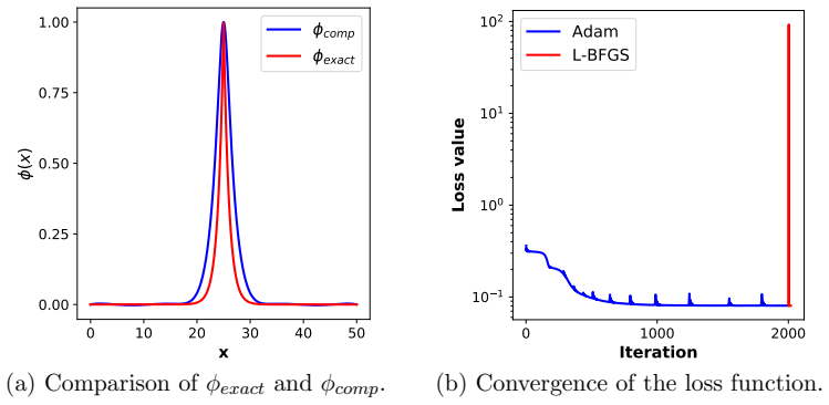
The central claim, stated on the paper's own terms, is that a deep neural network can approximate the solution of a boundary value problem in computational mechanics by minimizing the system's total potential energy rather than the residual of the strong-form PDE. The energy is taken as the loss function, Neumann (traction) conditions arise naturally from the variational principle, and Dirichlet conditions are built into the trial function, so no labeled data, mesh, or explicit weak-form derivation is needed. The paper demonstrates this Deep Energy Method on plane-stress and three-dimensional linear elasticity, hyperelastic torsion, phase-field fracture, piezoelectric coupling, and Kirchhoff plate bending, reporting relative $L^2$ displacement errors below about 2% for the classical elastic benchmarks and a 2.88% error on a 1D phase-field crack profile versus 70.6% for collocation. The authors present the method as a proof of concept that DNNs can serve as the approximation space in computational mechanics when the loss is the energy.

Load-bearing premise

The discrete sum over sampling points is assumed to be a faithful quadrature of the energy integral, so that minimizing it yields a function close to the true energy minimizer; the paper does not analyze this quadrature error and even notes that point sampling affects the stability and accuracy of the method for the annular plate.

Editorial extensions

If this is right

Mechanical boundary value problems become mesh-free: no mesh generation or element quadrature is required, only evaluation points in the domain.
No labeled data or external simulation is needed for training; the energy functional and boundary conditions are the only problem data, so the approach transfers to new materials or loads by changing the energy.
Natural (traction) boundary conditions are satisfied automatically through the variational principle, while essential (Dirichlet) conditions are built into the trial function, simplifying the loss.
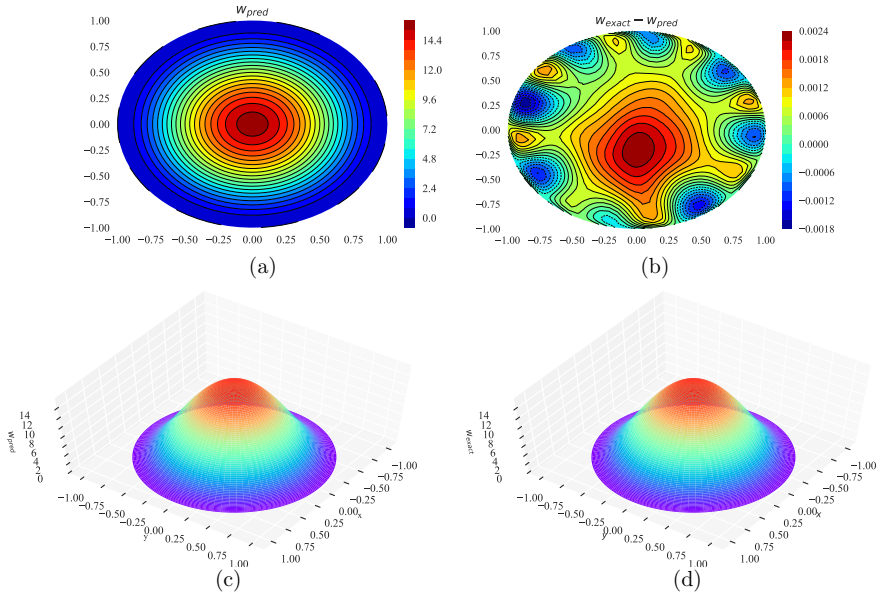
Fourth-order problems like Kirchhoff plate bending bypass the $C^1$-continuity requirement that complicates mesh-based methods, because the network and automatic differentiation provide smooth derivatives.
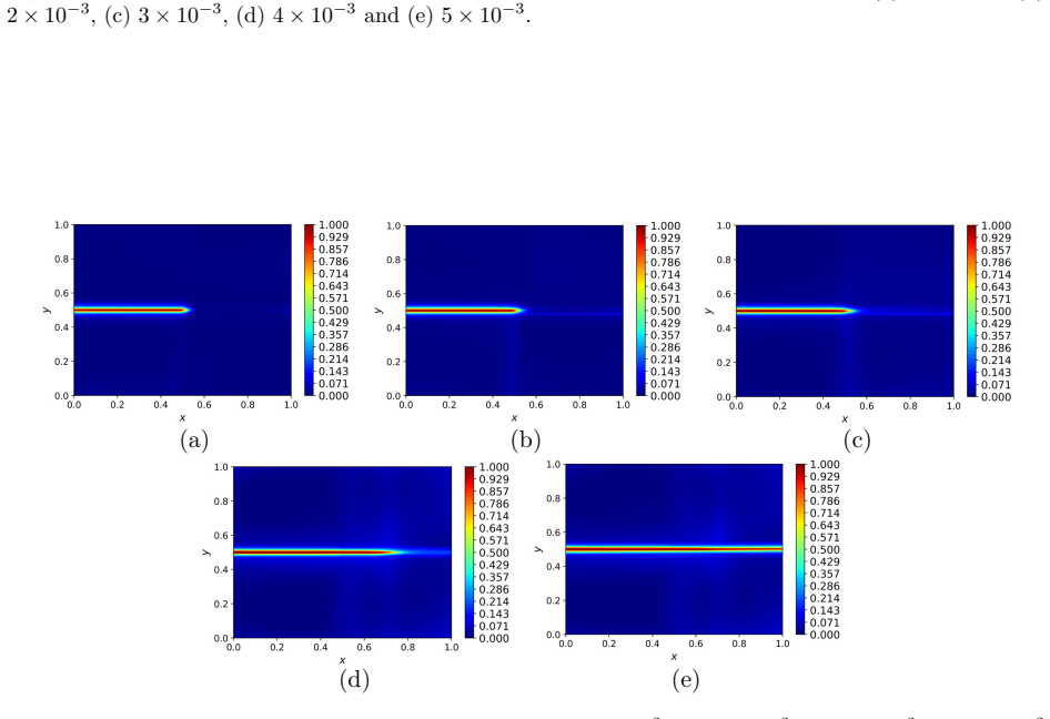
For phase-field fracture, the energy formulation captures the sharp crack profile far more accurately than collocation with the same architecture, pointing toward fracture simulation without remeshing.

Reading between the lines

Editorial extensions of the paper, not claims the author makes directly.

The reported accuracy depends on the sampling points acting as a quadrature rule; an obvious extension the paper leaves implicit is adaptive or error-driven point placement, which could make DEM robust on domains with stress concentrations or cutouts.
The same energy-as-loss principle should extend to dissipative or rate-dependent problems by using incremental potentials or rate functionals, though the paper only treats conservative systems.
Because a trained network gives a differentiable field at arbitrary query points, DEM could be paired with inverse problems or design loops that repeatedly evaluate stresses, a use not explored here.
A direct testable extension compares DEM's convergence rate against FEM on a problem with a known singular solution; if the quadrature is adequate, the energy minimizer should converge at a rate governed by network expressiveness and optimizer performance.

Share X Bluesky LinkedIn Reddit HN

Signed reviews

No signed human review yet.

Editorial analysis

A structured set of objections, weighed in public.

Desk editor's note, referee report, and a circularity audit.

Desk Editor's Note

read the letter

Quick take: this is a useful application paper built on Deep Ritz, not a new method; treat the phase-field and Neumann-boundary equations as needing correction before the headline numbers can be trusted. What's actually new: the energy-as-loss idea is E et al.'s Deep Ritz method [14], properly cited. The contribution is the breadth of computational mechanics applications: linear elasticity with internal pressure, hyperelastic torsion, phase-field fracture, piezoelectricity, and Kirchhoff plates with an autoencoder and problem-specific sinusoidal activation. That is a genuinely useful proof-of-concept collection, and the DEM-vs-collocation comparison for the 1D phase-field problem is instructive. What it does well: the linear elasticity benchmarks (0.5% for the cylinder, 1.8% for the plate with hole, 5.3% strain-energy error for the cube) are validated against analytical solutions and are plausible. The hyperelastic example is checked against a FEniCS reference. The paper is transparent about implementation details, gives code snippets, and explicitly acknowledges remaining caveats, including non-convexity and the sensitivity of the energy method to point sampling in Section 6.7.4. The soft spots are real but not all equal. The stress-test note lands: Eq. (77)-(78) define a 1D phase-field DEM loss that is not the phase-field energy used elsewhere in the paper; its Euler-Lagrange equation is a simple parabola, not the exponential profile of Eq. (71). As written, the reported 2.88% L2 error does not test the method as stated. Likewise, Eq. (28) defines the Neumann loss as a sum of tractions without a displacement multiplier, so it is dimensionally inconsistent with an external-work term. These look like typos, but the paper cannot be reproduced from the printed equations until they are fixed. The B parameter in Eq. (70) is self-referential, and the paper offers no quadrature error analysis for the discrete loss; Section 6.7.4 concedes that sampling affects stability and accuracy. No code or seeds are released, and repeated-run variance is not reported. Overall: the central idea is not new but is sound, and the applications are worth having. The paper deserves a serious referee, but the authors need to correct the phase-field energy, fix the Neumann loss, and release code before the quantitative claims can be accepted.

Referee Report

4 major / 4 minor

Summary. The paper proposes and tests the Deep Energy Method (DEM), in which the total potential energy of a mechanical system is used as the loss function for a fully connected deep neural network. The authors argue that, for problems with a variational structure, minimizing the empirical energy (Eq. 12) yields an approximate solution without meshes or labeled data. They present proof-of-concept applications in linear elasticity (pressurized cylinder, plate with a hole, hollow sphere, cube with a spherical hole), elastodynamics via collocation, hyperelasticity, phase-field fracture, piezoelectricity, and Kirchhoff plate bending. Benchmarks with analytical or finite-element reference solutions report relative L2 errors of about 0.5% to 5% for displacements and energies, and the paper contrasts DEM with deep collocation on several examples.

Significance. If the reported results are reproducible, DEM is a valuable extension of the physics-informed neural network literature into computational mechanics, particularly because it replaces residual-based losses with energy minimization and handles natural boundary conditions in a unified way. The paper's breadth—2D/3D linear elasticity, hyperelastic torsion, phase-field fracture, piezoelectricity, and fourth-order plate problems—goes well beyond most existing PINN studies and includes comparisons with analytical and finite-element solutions. The inclusion of code snippets and detailed architecture/optimizer specifications is helpful for reproducibility. However, several printed loss function definitions are not the mechanical energies they claim to be, and the discrete quadrature underlying Eq. (12) is not analyzed. These issues directly affect the quantitative claims and must be corrected before the results can be fully accepted.

major comments (4)

[6.5.1, Eqs. (77)-(78)] The functional being minimized in the one-dimensional phase-field DEM example is not the phase-field energy. As written, I(phi) = (1/2)∫(phi - l0^2 |∇phi|^2) dx, whose Euler-Lagrange equation is 1 + 2 l0^2 phi'' = 0, not the phase-field equilibrium equation in Eqs. (72)-(73) and not the Griffith-type energy in Eqs. (65) or (79). The reported 2.88% L2 error for DEM therefore does not test the energy method as stated, and the comparison with the 70.6% collocation error is not a valid demonstration for this benchmark. The functional must be corrected, or the relation of the printed functional to the phase-field energy must be explained.
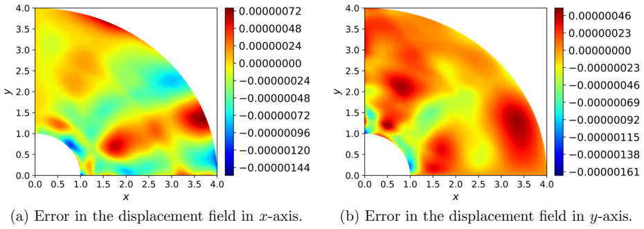
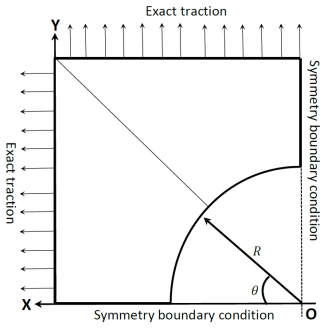
[6.2.1, Eq. (28); 6.2.2; 6.2.3, Eqs. (37), (40)] The Neumann boundary loss Lneu is not the work of external traction: fneu is defined as t_N,x + t_N,y (plus t_N,z in 3D) with no factor of the displacement, and it is weighted by the area/volume of the whole domain rather than by the boundary length/area. In the pressurized cylinder example, Eq. (26) defines t_N,x = P u and t_N,y = P v, so the traction itself depends on the unknown displacement, and the total loss Lint - Lneu is not the total potential energy of the system. As a result, the reported 0.5% and 1.8% displacement errors for the cylinder and plate-with-hole benchmarks are not tied to the minimization problem that the paper claims to solve. These equations need to be rewritten or clarified.
[4.2, Eq. (12); 6.7.4] The paper does not provide a quadrature error analysis or convergence study for the replacement of the energy integral by a weighted sum over sample points. This is load-bearing because if the sum is not an accurate quadrature, the network minimizes a different functional from the physical energy. The paper itself states in Section 6.7.4 that point sampling 'affects the stability and accurate of this deep energy method' and that a particular collocation point distribution was needed for the annular plate. A systematic study of the discrete loss as a function of the number and distribution of sampling points is needed to support the general claims made for DEM.
[6.5, Eq. (70)] The initial history amplitude is defined by B = 1/(1 - phi) for phi < 1, but phi is the unknown phase field that the method is supposed to compute. This makes H(x,0) in Eq. (69) depend on the solution before it is known, which is a circular definition. The authors should state how B is evaluated in practice, for example using an initial guess or a previous iteration, and whether the reported results are sensitive to that choice.

minor comments (4)

[6.2.1, Eq. (25)] In the analytical solution for the pressurized cylinder, the expression for vexact is printed as urad cos(theta), which is the same as uexact; it should presumably be urad sin(theta).
[6.2.1, 6.2.2] The text refers to the linear-elastic minimization problem as 'Eq. (65)', but Eq. (65) is the phase-field energy; the intended reference is likely the problem statement in Eq. (24).
[6.2.1, Eq. (28)] In Eq. (28), the boundary term uses A_Omega, the area of the domain, as the quadrature weight; for a line boundary in 2D this should be the length of the boundary (or the appropriate boundary measure), as is done for the volume versus surface terms in Eq. (37).
[6.7.4] The sentence 'the proper point sampling inside physical domain affects the stability and accurate of this deep energy method' should read 'affects the stability and accuracy', and the paragraph would benefit from a quantitative description of the sampling strategy used for the annular plate and of its effect on the reported errors.

Circularity Check

1 steps flagged · score 2.0 of 10

Central DEM validation is self-contained; one local self-referential definition appears in the phase-field crack initialization (B = 1/(1-φ)).

self definitional [Section 6.5, Eq. (70), used in Eqs. (69) and (79)]
"where B is a scalar parameter that controls the magnitude of the scalar history field and is calculated as: B = 1/(1−φ) for φ< 1."

Equations (69) and (79) use H(x,0), the initial strain-history field, as an input that determines the phase field φ through energy minimization. Equation (70) defines the scaling B of that input as 1/(1−φ), i.e., in terms of the very field φ being solved for. Since the degradation function is g(φ) = (1−φ)^2, the term g(φ)H(x,0) in the loss becomes (1−φ)·(...), so the 'initial condition' H is a function of the unknown output. The paper does not specify a fixed-point iteration, an initial guess for φ, or a separate representative value for φ that would make the definition well-posed; as written, the initialization step is self-referential. This is a narrow defect in one example, not in the central DEM derivation.

full rationale

The central claim—that minimizing a neural-network surrogate of the potential energy solves the benchmark BVPs—is not circular: for the linear-elastic cylinder, plate-with-hole, sphere, hyperelastic cuboid, piezoelectric beam, and Kirchhoff plates, the loss is built from the stated energy functional and the reported errors are measured against external analytical or FEM reference solutions. No parameter is fitted to those reference solutions, and no load-bearing premise rests on a self-citation. The one genuine circular step is local to the phase-field initialization: Eq. (70) defines B via the unknown φ, so H(x,0) in Eq. (69)—an input to the phase-field energy in Eq. (79)—depends on the solution φ being computed. This makes the initial-crack prediction self-referential as printed, though it does not infect the cylinder/plate/sphere benchmarks or the energy-method concept itself. Other apparent inconsistencies (e.g., the 1D phase-field functional in Eq. (77) not matching Eq. (65), and the Neumann-loss definitions in Eqs. (26)/(28)) are internal-consistency/correctness issues rather than input/output circularity; they should be treated as reproducibility risks, not as further circularity.

Assumptions & free parameters 5 free parameters · 5 assumptions · 0 invented entities

The central claim rests on standard calculus of variations, plus three domain assumptions the paper does not prove: uniform quadrature accuracy, success of non-convex optimization, and admissibility of the trial functions. The phase-field initialization introduces a self-referential parameter B. No new physical entities are introduced; the autoencoder and tailored activation functions are numerical constructs.

free parameters (5)

B (phase-field history amplitude) = B = 1/(1-φ) for φ < 1
Eq. (70). B controls H(x,0) in Eq. (69) but depends on the unknown phase-field φ, making the initial crack setup self-referential.
Neural network depth and width = e.g., 3x30, 3x50, 5x50, 3x150 neurons depending on example
Chosen by hand per benchmark in Section 6; no sensitivity study or selection rule.
Optimizer hyperparameters = Adam then L-BFGS; learning rate r=0.5 for L-BFGS in Section 6.4
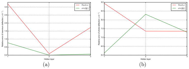
Manual configuration; non-convex optimization success depends on these choices.
Activation function for plate problems = sin(πx/2) instead of tanh
Section 6.7.3: activation 'tailored accordingly' because it improved accuracy on the benchmark; ad hoc model selection.
Collocation/sampling distribution for annular plate = 1000 points as in Fig. 33
Section 6.7.4: suitable sampling was discovered during numerical experiments; affects stability and accuracy.

assumptions (5)

standard math The variational energy E[u] has a unique minimizer equal to the solution of the strong form (Euler-Lagrange equivalence).
Section 2.2, Eqs. (6)-(7): the whole method assumes the minimizer of the energy is the PDE solution.
domain assumption The weighted sum over uniform collocation points accurately approximates the energy integral.
Eqs. (12) and (59); no quadrature error analysis is provided and Section 6.7.4 shows sensitivity to point placement.
domain assumption Gradient-based optimization of the non-convex finite-sum loss reaches an acceptable minimum.
Section 4.2.1 introduces the non-convex problem; Section 7 admits this is an unresolved caveat.
domain assumption The chosen trial functions with enforced Dirichlet BCs are sufficiently expressive and admissible.
Examples in Section 6 (e.g., u=x(1-x)uhat, phi trial in Eq. 74) constrain the DNN output; if the true solution cannot be represented in this form, the approach fails.
standard math Automatic differentiation computes the required derivatives correctly.
Used throughout Section 5 to build the energy and gradients; standard in TensorFlow/PyTorch.

how reviews work

0 comments

Cite this review

Pith. "Pith review of An Energy Approach to the Solution of Partial Differential Equations in Computational Mechanics via Machine Learning: Concepts, Implementation and Applications." pith.science (2026). https://pith.science/paper/WRDNUAJK

@misc{pith2026190810407,
  author       = {Pith},
  title        = {Pith review of: An Energy Approach to the Solution of Partial Differential Equations in Computational Mechanics via Machine Learning: Concepts, Implementation and Applications},
  year         = {2026},
  howpublished = {\url{https://pith.science/paper/WRDNUAJK}},
  note         = {Machine review of arXiv:1908.10407}
}

read the original abstract

Partial Differential Equations (PDE) are fundamental to model different phenomena in science and engineering mathematically. Solving them is a crucial step towards a precise knowledge of the behaviour of natural and engineered systems. In general, in order to solve PDEs that represent real systems to an acceptable degree, analytical methods are usually not enough. One has to resort to discretization methods. For engineering problems, probably the best known option is the finite element method (FEM). However, powerful alternatives such as mesh-free methods and Isogeometric Analysis (IGA) are also available. The fundamental idea is to approximate the solution of the PDE by means of functions specifically built to have some desirable properties. In this contribution, we explore Deep Neural Networks (DNNs) as an option for approximation. They have shown impressive results in areas such as visual recognition. DNNs are regarded here as function approximation machines. There is great flexibility to define their structure and important advances in the architecture and the efficiency of the algorithms to implement them make DNNs a very interesting alternative to approximate the solution of a PDE. We concentrate in applications that have an interest for Computational Mechanics. Most contributions that have decided to explore this possibility have adopted a collocation strategy. In this contribution, we concentrate in mechanical problems and analyze the energetic format of the PDE. The energy of a mechanical system seems to be the natural loss function for a machine learning method to approach a mechanical problem. As proofs of concept, we deal with several problems and explore the capabilities of the method for applications in engineering.

Figures

Figures reproduced from arXiv: 1908.10407 by the authors.

**Figure 2.** Error plots for pressurized thick-cylinder. [PITH_FULL_IMAGE:figures/full_fig_p013_2.png] view at source ↗

**Figure 3.** Problem setup for the plate with a circular hole example [PITH_FULL_IMAGE:figures/full_fig_p014_3.png] view at source ↗

Figures from the paper (32 more)

**Figure 4.** Figure 4: Computed solution and errors for plate with hole. [PITH_FULL_IMAGE:figures/full_fig_p015_4.png]

**Figure 5.** Figure 5: Geometrical Setup and boundary condition for the application of linear elasticity on three [PITH_FULL_IMAGE:figures/full_fig_p016_5.png]

**Figure 6.** Figure 6: Computed solution for the hollow sphere subjected to internal pressure [PITH_FULL_IMAGE:figures/full_fig_p017_6.png]

**Figure 7.** Figure 7: Computed solution for the cube with a hole example [PITH_FULL_IMAGE:figures/full_fig_p018_7.png]

**Figure 8.** Figure 8: Comparison between the computed and exact solutions for the 1D wave propagation example [PITH_FULL_IMAGE:figures/full_fig_p019_8.png]

**Figure 9.** Figure 9: Motion of body B. rather than the strong formulation. The potential functional is written as E(ϕ) = Z Ω Ψ dV − Z Ω fb · ϕ dV − Z ∂ΩN t · ϕ dA. (55) In order to obtain the solution we minimize the potential energy min ϕ∈H E(ϕ), (56) where H is the set of admissible func…

**Figure 10.** Figure 10: A hyperelastic 3D Cuboid is twisted an angle of 60 [PITH_FULL_IMAGE:figures/full_fig_p022_10.png]

**Figure 11.** Figure 11: The training point distribution of a 3D hyperelastic cuboid in DEM. The red points correspond [PITH_FULL_IMAGE:figures/full_fig_p023_11.png]

**Figure 12.** Figure 12: Positions of AB line and CDEF plane. (a) Displacement comparison (b) Stress comparison [PITH_FULL_IMAGE:figures/full_fig_p024_12.png]

**Figure 13.** Figure 13: The displacement and stress results of DEM measured at the AB line compared to the reference [PITH_FULL_IMAGE:figures/full_fig_p024_13.png]

**Figure 14.** Figure 14: Displacement and VonMises stress at the CDEF plane in DEM of a twisted Neo-Hookean 3D [PITH_FULL_IMAGE:figures/full_fig_p025_14.png]

**Figure 15.** Figure 15: One-dimensional phase field model using the collocation method. [PITH_FULL_IMAGE:figures/full_fig_p028_15.png]

**Figure 16.** Figure 16: One-dimensional phase field model using the energy method. [PITH_FULL_IMAGE:figures/full_fig_p029_16.png]

**Figure 17.** Figure 17: Single-edge notch tension example. 29 [PITH_FULL_IMAGE:figures/full_fig_p029_17.png]

**Figure 18.** Figure 18: Initialization of crack in the plate using the strain-history function. [PITH_FULL_IMAGE:figures/full_fig_p031_18.png]

**Figure 19.** Figure 19: Scatter plots of the deformed configuration for prescribed displacement of (a) 1 [PITH_FULL_IMAGE:figures/full_fig_p033_19.png]

**Figure 20.** Figure 20: Crack pattern for prescribed displacement of (a) 1 [PITH_FULL_IMAGE:figures/full_fig_p033_20.png]

**Figure 21.** Figure 21: Schematic diagram showing the electrical and the mechanical boundary conditions for the can [PITH_FULL_IMAGE:figures/full_fig_p035_21.png]

**Figure 22.** Figure 22: The predicted values of three outputs of the system using DEM: (a) applying mechanical loading, [PITH_FULL_IMAGE:figures/full_fig_p035_22.png]

**Figure 24.** Figure 24: (a) Predicted deflection contour (b) Deflection error contour (c) Predicted deflection (d) Analytical deflection of the simply-supported plate on Winkler foundation with 3 hidden layers and 50 neurons. layer and neuron number grows, the maximum deflection becomes more…

**Figure 26.** Figure 26: (a) Predicted deflection contour (b) Deflection error contour (c) Predicted deflection (d) Exact deflection of the clamped circular plate with 3 hidden layers and 50 neurons 41 [PITH_FULL_IMAGE:figures/full_fig_p041_26.png]

**Figure 27.** Figure 27: Relative error of (a) maximum deflection and (b) whole deflection predicted by Tanh and proposed activation function of a DNN for the simply-supported plate 1 2 3 Hidden layer 0.0 0.5 1.0 1.5 2.0 2.5 3.0 R elativ e error of m a x mium defle ction (x10¡5) Tanh(x) sin( …

**Figure 28.** Figure 28: Relative error of (a) maximum deflection and (b) whole deflection predicted by Tanh and proposed activation function of a DNN with an autoencoder for the simply-supported plate 10 15 20 25 30 35 40 45 50 Neurons per hidden layer 0 1 2 3 4 5 6 7 R elativ e error of m a…

**Figure 29.** Figure 29: Relative error of (a) maximum deflection and (b) whole deflection predicted by different encoding layer configurations of a DNN with an autoencoder for the simply-supported plate. 43 [PITH_FULL_IMAGE:figures/full_fig_p043_29.png]

**Figure 30.** Figure 30: The computational time of ten encoding layer configurations for the autoencoder [PITH_FULL_IMAGE:figures/full_fig_p044_30.png]

**Figure 31.** Figure 31: Relative error of (a) deflection and (b) predicted by the DNN with an autoencoder and IGA for the simply-supported plate. 44 [PITH_FULL_IMAGE:figures/full_fig_p044_31.png]

**Figure 32.** Figure 32: (a) Predicted deflection contour (b) Deflection error contour (c) Predicted deflection (d) Analytical deflection of the simply-supported square plate. contour error plot of deflection predicted by two encoding layers with [150,100] neurons are shown in [PITH_FULL_IMA…

**Figure 33.** Figure 33: Collocation points in the annular domain. [PITH_FULL_IMAGE:figures/full_fig_p046_33.png]

**Figure 34.** Figure 34: Relative error of (a) maximum deflection and (b) whole deflection predicted by tanh and proposed activation function of a DNN for the annular plate. with an autoencoder is also constructed which will help better predict the physical pattern of this problem. During our…

**Figure 35.** Figure 35: Relative error of (a) maximum deflection and (b) whole deflection predicted by different encoding layer configurations of a DNN with an autoencoder for the simply-supported plate. [1] [2] [3] [2 1] [3 1] [3 2] [3 2 1] 0 20 40 60 80 100 120 140 160 Computation Time (s)…

**Figure 36.** Figure 36: The computational time of seven encoding layer configurations for the autoencoder. [PITH_FULL_IMAGE:figures/full_fig_p047_36.png]

**Figure 37.** Figure 37: (a) Predicted deflection contour (b) Deflection error contour (c) Predicted deflection (d) Analytical deflection of the simply-supported annular plate with 3 hidden layers and 50 neurons. Additionally, the deflection contour and the error contour are also shown in [P…

Discussion (0). Continue with ORCID to comment.

Reference graph

Works this paper leans on

38 extracted references · 28 canonical work pages

[14]

Weinan, B

E. Weinan, B. Yu, The deep ritz method: A deep learning-based numerical algorithm for solving variational problems, Communications in Mathematics and Statistics 6 (1) (2018) 1–12

2018
[1]

T. J. Hughes, The ﬁnite element method: linear static and dynamic ﬁnite element analysis, Courier Corporation, 2012

work page 2012
[2]

Huerta, T

A. Huerta, T. Belytschko, S. Fern´ andez-M´ endez, T. Rabczuk, X. Zhuang, M. Arroyo, Meshfree methods, Encyclopedia of Computational Mechanics Second Edition (2018) 1–38

work page 2018
[3]

T. J. Hughes, G. Sangalli, M. Tani, Isogeometric analysis: Mathematical and imple- mentational aspects, with applications, in: Splines and PDEs: From Approximation Theory to Numerical Linear Algebra, Springer, 2018, pp. 237–315

work page 2018
[4]

Goodfellow, Y

I. Goodfellow, Y. Bengio, A. Courville, Deep learning, MIT press, 2016

2016
[5]

Abadi, P

M. Abadi, P. Barham, J. Chen, Z. Chen, A. Davis, J. Dean, M. Devin, S. Ghemawat, G. Irving, M. Isard, et al., Tensorﬂow: A system for large-scale machine learning, in: 12th {USENIX} Symposium on Operating Systems Design and Implementation ({OSDI} 16), 2016, pp. 265–283

work page 2016
[6]

Ketkar, Introduction to pytorch, in: Deep learning with python, Springer, 2017, pp

N. Ketkar, Introduction to pytorch, in: Deep learning with python, Springer, 2017, pp. 195–208

work page 2017
[7]

M. S. Alnæs, A. Logg, K. B. Ølgaard, M. E. Rognes, G. N. Wells, Uniﬁed form language: A domain-speciﬁc language for weak formulations of partial diﬀerential equations, ACM Transactions on Mathematical Software (TOMS) 40 (2) (2014) 9

work page 2014

Show all 38 references

[8]

Raissi, Deep hidden physics models: Deep learning of nonlinear partial diﬀerential equations, The Journal of Machine Learning Research 19 (1) (2018) 932–955

M. Raissi, Deep hidden physics models: Deep learning of nonlinear partial diﬀerential equations, The Journal of Machine Learning Research 19 (1) (2018) 932–955

2018
[9]

Raissi, P

M. Raissi, P. Perdikaris, G. E. Karniadakis, Physics informed deep learning (part i): Data-driven solutions of nonlinear partial diﬀerential equations, arXiv preprint arXiv:1711.10561

arXiv
[10]

Dacorogna, Introduction to the Calculus of Variations, World Scientiﬁc Publishing Company, 2014

B. Dacorogna, Introduction to the Calculus of Variations, World Scientiﬁc Publishing Company, 2014

2014
[11]

Baiges, R

J. Baiges, R. Codina, I. Castanar, E. Castillo, A ﬁnite element reduced order model based on adaptive mesh reﬁnement and artiﬁcial neural networks. 49
[12]

Kirchdoerfer, M

T. Kirchdoerfer, M. Ortiz, Data-driven computational mechanics, Computer Methods in Applied Mechanics and Engineering 304 (2016) 81–101

2016
[13]

Ruthotto, E

L. Ruthotto, E. Haber, Deep Neural Networks Motivated by Partial Diﬀerential Equa- tions, arXiv e-print 1804.04272

arXiv
[15]

L. Lei, C. Ju, J. Chen, M. I. Jordan, Non-convex ﬁnite-sum optimization via scsg methods, in: Advances in Neural Information Processing Systems, 2017, pp. 2348–2358

2017
[16]

Petersen, M

P. Petersen, M. Raslan, F. Voigtlaender, Topological properties of the set of functions generated by neural networks of ﬁxed size, arXiv preprint arXiv:1806.08459

arXiv
[17]

M. I. Jordan, Dynamical, symplectic and stochastic perspectives on gradient-based op- timization, University of California, Berkeley
[18]

Glorot, Y

X. Glorot, Y. Bengio, Understanding the diﬃculty of training deep feedforward neu- ral networks, in: Proceedings of the thirteenth international conference on artiﬁcial intelligence and statistics, 2010, pp. 249–256

2010
[19]

Abadi, A

M. Abadi, A. Agarwal, P. Barham, E. Brevdo, Z. Chen, C. Citro, G. S. Corrado, A. Davis, J. Dean, M. Devin, et al., Tensorﬂow: Large-scale machine learning on het- erogeneous distributed systems, arXiv preprint arXiv:1603.04467

arXiv
[20]

J. He, L. Li, J. Xu, C. Zheng, Relu deep neural networks and linear ﬁnite elements, arXiv preprint arXiv:1807.03973

arXiv
[21]

Opschoor, P

J. Opschoor, P. Petersen, C. Schwab, Deep relu networks and high-order ﬁnite element methods, SAM, ETH Z¨ urich
[22]

Y. Jia, C. Anitescu, Y. J. Zhang, T. Rabczuk, An adaptive isogeometric analysis col- location method with a recovery-based error estimator, Computer Methods in Applied Mechanics and Engineering 345 (2019) 52–74

2019
[23]

S. P. Timoshenko, J. Goodier, Theory of elasticity, McGraw-hill, 1970

1970
[24]

Avrutskiy, Enhancing approximation abilities of neural networks by training deriva- tives, arXiv preprint arXiv:1712.04473

V. Avrutskiy, Enhancing approximation abilities of neural networks by training deriva- tives, arXiv preprint arXiv:1712.04473

arXiv
[25]

J. Berg, K. Nystr¨ om, A uniﬁed deep artiﬁcial neural network approach to partial dif- ferential equations in complex geometries, Neurocomputing 317 (2018) 28–41

2018
[26]

P. L. Gould, Y. Feng, Introduction to linear elasticity, Springer, 1994

1994
[27]

Schillinger, J

D. Schillinger, J. A. Evans, F. Frischmann, R. R. Hiemstra, M.-C. Hsu, T. J. Hughes, A collocated c0 ﬁnite element method: Reduced quadrature perspective, cost comparison with standard ﬁnite elements, and explicit structural dynamics, International Journal for Numerical Method...

2015
[28]

M. A. Scott, R. N. Simpson, J. A. Evans, S. Lipton, S. P. Bordas, T. J. Hughes, T. W. Sederberg, Isogeometric boundary element analysis using unstructured t-splines, Computer Methods in Applied Mechanics and Engineering 254 (2013) 197–221

2013
[29]

Logg, K.-A

A. Logg, K.-A. Mardal, G. Wells, Automated solution of diﬀerential equations by the ﬁnite element method: The FEniCS book, Vol. 84, Springer Science & Business Media, 2012

2012
[30]

Bourdin, G

B. Bourdin, G. Francfort, J.-J. Marigo, Numerical experiments in revisited brittle fracture, Journal of the Mechanics and Physics of Solids 48 (4) (2000) 797–826. doi:10.1016/S0022-5096(99)00028-9

2000 doi
[31]

Griﬃth, The Phenomena of Rupture and Flow in Solids, Philisophical Transactions of the Royal Society of London 221 (Series A) (1921) 163–198

A. Griﬃth, The Phenomena of Rupture and Flow in Solids, Philisophical Transactions of the Royal Society of London 221 (Series A) (1921) 163–198

1921
[32]

M. J. Borden, T. J. Hughes, C. M. Landis, C. V. Verhoosel, A higher-order phase-ﬁeld model for brittle fracture: Formulation and analysis within the isogeometric analysis framework, Computer Methods in Applied Mechanics and Engineering 273 (2014) 100–

2014
[33]

Miehe, F

C. Miehe, F. Welschinger, M. Hofacker, Thermodynamically consistent phase-ﬁeld models of fracture: Variational principles and multi-ﬁeld FE implementations, Inter- national Journal for Numerical Methods in Engineering 83 (10) (2010) 1273–1311. doi:10.1002/nme.2861

2010 doi
[34]

Miehe, M

C. Miehe, M. Hofacker, F. Welschinger, A phase ﬁeld model for rate-independent crack propagation: Robust algorithmic implementation based on operator splits, Computer Methods in Applied Mechanics and Engineering 199 (45-48) (2010) 2765–2778. doi: 10.1016/J.CMA.2010.04.011

2010 doi
[35]

M. J. Borden, C. V. Verhoosel, M. A. Scott, T. J. Hughes, C. M. Landis, A phase-ﬁeld description of dynamic brittle fracture, Computer Methods in Applied Mechanics and Engineering 217-220 (2012) 77–95. doi:10.1016/J.CMA.2012.01.008

2012 doi
[36]

S. P. Timoshenko, S. Woinowsky-Krieger, Theory of plates and shells, McGraw-hill, 1959

1959
[37]

V. P. Nguyen, C. Anitescu, S. P. Bordas, T. Rabczuk, Isogeometric analysis: an overview and computer implementation aspects, Mathematics and Computers in Simulation 117 (2015) 89–116. 51

2015
[118]

doi:10.1016/J.CMA.2014.01.016

2014 doi

Pith tools

Reviewed August 14, 2026 · model on record in the stance chip above.

[1] [14]

Weinan, B

E. Weinan, B. Yu, The deep ritz method: A deep learning-based numerical algorithm for solving variational problems, Communications in Mathematics and Statistics 6 (1) (2018) 1–12

2018

[2] [1]

T. J. Hughes, The ﬁnite element method: linear static and dynamic ﬁnite element analysis, Courier Corporation, 2012

work page 2012

[3] [2]

Huerta, T

A. Huerta, T. Belytschko, S. Fern´ andez-M´ endez, T. Rabczuk, X. Zhuang, M. Arroyo, Meshfree methods, Encyclopedia of Computational Mechanics Second Edition (2018) 1–38

work page 2018

[4] [3]

T. J. Hughes, G. Sangalli, M. Tani, Isogeometric analysis: Mathematical and imple- mentational aspects, with applications, in: Splines and PDEs: From Approximation Theory to Numerical Linear Algebra, Springer, 2018, pp. 237–315

work page 2018

[5] [4]

Goodfellow, Y

I. Goodfellow, Y. Bengio, A. Courville, Deep learning, MIT press, 2016

2016

[6] [5]

Abadi, P

M. Abadi, P. Barham, J. Chen, Z. Chen, A. Davis, J. Dean, M. Devin, S. Ghemawat, G. Irving, M. Isard, et al., Tensorﬂow: A system for large-scale machine learning, in: 12th {USENIX} Symposium on Operating Systems Design and Implementation ({OSDI} 16), 2016, pp. 265–283

work page 2016

[7] [6]

Ketkar, Introduction to pytorch, in: Deep learning with python, Springer, 2017, pp

N. Ketkar, Introduction to pytorch, in: Deep learning with python, Springer, 2017, pp. 195–208

work page 2017

[8] [7]

M. S. Alnæs, A. Logg, K. B. Ølgaard, M. E. Rognes, G. N. Wells, Uniﬁed form language: A domain-speciﬁc language for weak formulations of partial diﬀerential equations, ACM Transactions on Mathematical Software (TOMS) 40 (2) (2014) 9

work page 2014