REVIEW 3 major objections 3 minor 10 references
On the stability of optimization algorithms given by discretizations of the Euler-Lagrange ODE
T0 review · 3 major / 3 minor · reviewed 2026-08-14 · deepseek-v4-flash
Pith's one-line read The paper claims that a cheap explicit-implicit Euler discretization of the accelerated-optimization Euler-Lagrange ODE remains stable up to an explicit, parameter-dependent iteration bound.
desk verdict The central stability bound is unsupported—the proof in A.4 uses a necessary condition as if it were sufficient—and the paper needs major revision, though the implicit/explicit Euler analysis has some value. read the letter →
The pith
A machine-rendered reading of the paper's core claim, the machinery that carries it, and where it could break.
The reading
What carries the argument
The central object is the stability function $R(M_k)=|\lambda_{\max}(M_k)|$ and its limit $R(M_\infty)=\lim_{k\to\infty} R(M_k)$, which classifies end behavior: $R<1$ converges, $R=1$ is stable, and $R>1$ diverges. For the explicit-implicit method the iteration matrix is $$M_k=\begin{pmatrix} 1-a_k & a_k \\ -b_k+a_k b_k & 1-a_k b_k \end{pmatrix}$$ with $a_k=p/k$ and $b_k=C p \epsilon (k+1)^{p-1} A$. The proof computes its eigenvalues, reduces the divergence threshold to $y+\sqrt{y^2-4x}\le 4$ with $x=a_k b_k$ and $y=x+a_k$, and then converts the threshold into the iteration bound $a_k b_k<4$. A prior diagonalization step justifies doing the analysis in one dimension for a general symmetric positive definite $A$, and the bound is stated using the largest eigenvalue, the smoothness constant $L$.
What would settle it
Take a one-dimensional quadratic with $p=3$, $L=10$, $\delta=0.01$, choose $C<1/(\epsilon L)$, and evaluate the exact eigenvalues of $M_k$ at $k$ around $44,445$. If the exact stability inequality $y+\sqrt{y^2-4x}\le 4$ fails at or below the claimed bound (equivalently, $R(M_k)>1$), the theorem's guarantee is false; a direct run of the update equations would settle the question empirically.
Extended reading notes
Core claim
The central claim is that, for a strongly convex $L$-smooth quadratic $f$, the explicit-implicit Euler discretization of $$\ddot{X}_t + \frac{p+1}{t}\dot{X}_t + $Cp^{2}$ $t^{{p-2}}$\nabla f(X_t)=0$$ has a computable epoch of reliable behavior. For $p=2$ the spectral radius of the iteration matrix tends to $1$, so the iterates oscillate around the minimizer without diverging; for $p>2$, stability holds while $k<\left(\frac{4}{C L p^2 \epsilon}\right)^{1/(p-2)}$, with $\epsilon=\delta^p$, $\delta<1/L$, and $C<1/(\epsilon L)$. The authors derive this by writing the update as $[x_{k+1};\,z_{k+1}]=M_k[x_k;\,z_k]$, computing the eigenvalues of $M_k$, and identifying where the largest eigenvalue crosses magnitude $1$. They conclude from the same calculation that implicit Euler converges for all $p$ and explicit Euler diverges for all $p$.
Load-bearing premise
The result rests on assuming that a simplified product inequality is enough to guarantee stability, but the proof's triangle-inequality step only shows the reverse direction—that exact stability implies the simpler inequality—so the sufficiency of the simpler condition is the load-bearing unproved premise.
Editorial extensions
If this is right
- For $p>2$, a practitioner running the naive explicit-implicit discretization with $\delta<1/L$ is guaranteed stable behavior through roughly $(4/(C L p^2 \delta^p))^{1/(p-2)}$ iterations, after which divergence is possible.
- For $p=2$ the naive discretization is claimed not to diverge at all in the strongly convex quadratic setting, matching the stable end behavior of the underlying ODE.
- The implicit Euler discretization converges for every $p$ and appears numerically to keep the accelerated rate, but each step requires solving an implicit system, which is the practical obstacle.
- The explicit Euler discretization diverges for every $p$, so it cannot be used for long horizons; the explicit-implicit scheme is the recommended middle ground.
- In higher dimensions only the largest eigenvalue of $A$ enters the bound, so a single $L$-smoothness constant controls the stability window.
Reading between the lines
- The paper does not prove its bound is sharp; solving the exact threshold $y+\sqrt{y^2-4x}=4$ numerically would reveal how much conservatism the triangle-inequality simplification adds and whether the true divergence time is longer.
- For non-quadratic smooth objectives, linearizing $\nabla f$ at the current iterate turns the same one-dimensional spectral calculation into a local, iteration-dependent stability estimate, an extension the paper only mentions.
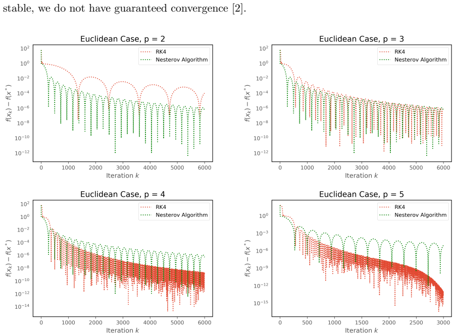
- The numerical observation that an explicit fourth-order Runge-Kutta discretization survives longer before diverging suggests the same stability-function analysis could bound Runge-Kutta variants.
- If the implicit Euler scheme's apparent acceleration holds in general, it offers a backward-stable route to realizing the $O(1/t^p)$ rate in discrete time; the paper reports the numerics but does not prove the rate.
Signed reviews
Editorial analysis
A structured set of objections, weighed in public.
Referee Report
Summary. The paper analyzes stability of Euler discretizations of the Euler-Lagrange ODE (1.2) used to model accelerated optimization methods. The central result is Theorem 3.1, which claims that for a strongly convex L-smooth quadratic objective, step size δ < 1/L, ε = δ^p, and C < 1/(εL), the explicit-implicit Euler discretization is stable for p = 2 and, for p > 2, exhibits stable behavior while k < (4/(CLp^2 ε))^{1/(p-2)}. The paper also analyzes the implicit Euler discretization (claimed converging) and the explicit Euler discretization (claimed diverging), with numerical experiments in Section 5.
Significance. The question addressed is of genuine interest: explaining and bounding the divergence of the naive discretization of the Wibisono et al. ODE could clarify when such discretizations are usable. The paper is clearly written, and the reduction to a scalar eigenvalue problem via eigendecomposition (Proposition 2.1) is standard and reasonable. However, the central stability bound is false as stated. I provide below an explicit parameter set satisfying every hypothesis of Theorem 3.1 for which the claimed bound holds while the iteration matrix has spectral radius greater than one. The flaw is not a minor technicality; it is a logical inversion in Appendix A.4 that invalidates Theorem 3.1(b). Because that theorem is the main contribution, the manuscript is not publishable in current form.
major comments (3)
- [Appendix A.4, Eq. (A.4)] Equation (A.4) gives the divergence condition y + sqrt(y^2 - 4x) > 4, where x = a_k b_k and y = x + a_k. The text then states that by the triangle inequality, y + s2 <= 4 implies s1 = 2 sqrt(x) < 4, and concludes that 'stability or convergence is achieved when s1 < 4.' This is a one-way implication: y + s2 <= 4 does imply s1 < 4, but s1 < 4 does not imply y + s2 <= 4 because y = x + a_k > x. The exact stability condition is not s1 < 4; it is y + sqrt(y^2 - 4x) <= 4. Thus the bound in Theorem 3.1(b) is derived from a necessary condition treated as sufficient. A concrete counterexample: take p = 3, A = L = 10, δ = 0.099, ε = δ^3, C = 5.73, and k = 4. All hypotheses of Theorem 3.1 are satisfied (δ < 1/L, k > p, C < 1/(εL)), and the claimed bound gives k < (4/(CLp^2 ε))^{1/(p-2)} = 8, so k = 4 is within the bound. For these parameters, a_k b_k ≈ 3.125 < 4, but y + sqrt(y^2 - 4x) ≈ 5.46 > 4; the matrix M_4 in Eq. (3.3) has eigenvalues approximately -0.14 and -1.73, so the spectral radius exceeds 1 and the iterates diverge. This directly contradicts Theorem 3.1(b).
- [Section A.2] The asymptotic analysis for p > 2 is not legitimate because the matrices M_k in Eq. (3.3) contain entries proportional to (k+1)^{p-1} and p/k; for p > 2 these entries do not converge to a finite matrix. The characteristic equation λ^2 + λ(c - 2) + 1 with c = lim_{k→∞} C p^2 ε k^{p-2} A therefore relies on a divergent limit, since c → ∞ when p > 2. This part of the proof should be revised or removed before any end-behavior claim for p > 2 can be made.
- [Abstract and Theorem 3.1(b)] The abstract states the stability bound as k < (4/(L p^2 δ^p))^{1/(p-2)}, without the constant C, while Theorem 3.1(b) states k < (4/(C L p^2 ε))^{1/(p-2)} with ε = δ^p. Since C is a free parameter subject only to C < 1/(εL), these are different claims and the discrepancy can be arbitrarily large. The statement of the main result must be internally consistent before the theorem can be evaluated.
minor comments (3)
- [Section 1.4, table] The notation 'p−2√' for the (p-2)-th root is confusing; it should be written as (·)^{1/(p-2)}.
- [Section 2, Definition 2.1 and Proposition 2.2] The definition of stability requires |x_k - x*| = |x_{k+1} - x*| for all sufficiently large k, but the proof of Proposition 2.2(b) only shows that the eigencomponent along an eigenvalue of magnitude 1 stays constant in magnitude. Complex conjugate eigenvalues on the unit circle rotate the vector, so the stated equality of consecutive absolute errors is not established.
- [Section 5.1, Figure 2] The tabulated bound 44,445 cannot be reproduced from the formulas in the abstract or Theorem 3.1 without specifying the value of C; with the abstract's formula the strict inequality gives 44,444 as the largest integer k for the stated parameters.
Circularity Check
No significant circularity: the stability analysis is derived analytically from the ODE and discretization, with no fitted prediction or load-bearing self-citation.
full rationale
The paper's derivation chain is self-contained in the relevant sense for circularity analysis. Theorem 3.1 is obtained by writing the explicit-implicit Euler discretization of the Euler-Lagrange ODE as the matrix iteration u_{k+1} = M_k u_k, computing the eigenvalues of M_k, and analyzing the stability function R(M_k). No parameter is fitted to data and then renamed as a prediction; the constants L, epsilon, delta, and C are inputs to a priori hypotheses, not calibrated outputs. The cited prior work ([8], Wibisono et al.) provides the continuous-time ODE itself, which is external to this paper and not invoked as a uniqueness theorem to forbid alternatives. The numerical experiments in Section 5 confirm the claimed bounds but do not supply the bound. The reader's take identifies a genuine proof gap in Appendix A.4: the implication 'y + s2 <= 4 implies s1 < 4' is used in the converse direction to conclude stability from s1 < 4, and the resulting bound is at best necessary rather than sufficient. However, a one-way implication or an invalid sufficiency argument is a correctness flaw, not circularity: it does not make the conclusion equivalent to an input by definition, nor does it fit an output to the data used to produce it. Therefore the appropriate circularity score is 0, with no circular steps to report.
Assumptions & free parameters
free parameters (1)
- C =
1 (in numerical experiments)
assumptions (4)
- domain assumption The Euler-Lagrange ODE (1.2) derived by Wibisono et al. correctly models accelerated optimization with O(1/t^p) rate.
- domain assumption The largest eigenvalue magnitude of the iteration matrix determines stability of the update sequence.
- ad hoc to paper The stability condition y + sqrt(y^2 - 4x) <= 4 can be replaced by 2 sqrt(x) < 4 as a sufficient condition.
- domain assumption Reduction to a one-dimensional quadratic problem is without loss of generality.
Cite this review
Pith. "Pith review of On the stability of optimization algorithms given by discretizations of the Euler-Lagrange ODE." pith.science (2026). https://pith.science/paper/IWXCF25I
@misc{pith2026190810426,
  author       = {Pith},
  title        = {Pith review of: On the stability of optimization algorithms given by discretizations of the Euler-Lagrange ODE},
  year         = {2026},
  howpublished = {\url{https://pith.science/paper/IWXCF25I}},
  note         = {Machine review of arXiv:1908.10426}
}
abstract
The derivation of second-order ordinary differential equations (ODEs) as continuous-time limits of optimization algorithms has been shown to be an effective tool for the analysis of these algorithms. Additionally, discretizing generalizations of these ODEs can lead to new families of optimization methods. We study discretizations of an Euler-Lagrange equation which generate a large class of accelerated methods whose convergence rate is $O(\frac{1}{t^p})$ in continuous-time, where parameter $p$ is the order of the optimization method. Specifically, we address the question asking why a naive explicit-implicit Euler discretization of this solution produces an unstable algorithm, even for a strongly convex objective function. We prove that for a strongly convex $L$-smooth quadratic objective function and step size $\delta<\frac{1}{L}$, the naive discretization will exhibit stable behavior when the number of iterations $k$ satisfies the inequality $k < (\frac{4}{Lp^2 \delta^p})^{\frac{1}{p-2}}$. Additionally, we extend our analysis to the implicit and explicit Euler discretization methods to determine end behavior.
Figures


Figures from the paper (2 more)

Reference graph
Works this paper leans on
-
[1]
Explicit Stabilised Gradient Descent for Faster Strongly Convex Optimisation
Armin Eftekhari, Bart Vandereycken, Gilles Vilmart, and Konstantinos C Zygalakis. Explicit sta- bilised gradient descent for faster strongly convex optimisation. arXiv preprint arXiv:1805.07199, 2018
work page Pith review arXiv 2018
-
[2]
Desmond J Higham and Lloyd N Trefethen. Stiffness of odes. BIT Numerical Mathematics , 33(2):285–303, 1993
work page 1993
-
[3]
A method for solving convex programming problems with convergence rate o(1/k2)
Y Nesterov. A method for solving convex programming problems with convergence rate o(1/k2). Soviet Mathematics Doklady , 27:367–372, 1983
work page 1983
-
[4]
Accelerating the cubic regularization of newton’s method on convex problems
Yu Nesterov. Accelerating the cubic regularization of newton’s method on convex problems. Mathematical Programming, 112(1):159–181, 2008
2008
-
[5]
Understanding the acceleration phenomenon via high-resolution differential equations
Bin Shi, Simon S Du, Michael I Jordan, and Weijie J Su. Understanding the acceleration phenomenon via high-resolution differential equations. arXiv preprint arXiv:1810.08907 , 2018
arXiv 2018
-
[6]
Acceleration via Symplectic Discretization of High-Resolution Differential Equations
Bin Shi, Simon S Du, Weijie J Su, and Michael I Jordan. Acceleration via symplectic discretization of high-resolution differential equations. arXiv preprint arXiv:1902.03694 , 2019
work page Pith review arXiv 1902
-
[7]
A differential equation for modeling nesterov’s accelerated gradient method: Theory and insights
Weijie Su, Stephen Boyd, and Emmanuel Candes. A differential equation for modeling nesterov’s accelerated gradient method: Theory and insights. In Advances in Neural Information Processing Systems, pages 2510–2518, 2014
work page 2014
-
[8]
Andre Wibisono, Ashia C. Wilson, and Michael I. Jordan. A variational perspective on accelerated methods in optimization. Proceedings of the National Academy of Sciences, 113(47):E7351–E7358, 2016
work page 2016
Show all 10 references
-
[9]
Direct runge-kutta discretization achieves acceleration
Jingzhao Zhang, Aryan Mokhtari, Suvrit Sra, and Ali Jadbabaie. Direct runge-kutta discretization achieves acceleration. In Advances in Neural Information Processing Systems , pages 3900–3909, 2018. 13 A Proof of Theorem 3.1 In Proposition 2.1, we showed that the case where x a...
2018
-
[10]
We have 0 = det(M∞−λI) = lim k→∞ det ( 1− p k−λ p k −Cpϵ(k + 1)p−1(k−p k )A 1−Cpϵ(k + 1)p−1(p k)A−λ ) =λ2 +λ(Cp2ϵA− 2) + 1 =λ2 +λ(4CϵA− 2) + 1
In the characteristic equation, we omit terms that go to 0 as k→∞ . We have 0 = det(M∞−λI) = lim k→∞ det ( 1− p k−λ p k −Cpϵ(k + 1)p−1(k−p k )A 1−Cpϵ(k + 1)p−1(p k)A−λ ) =λ2 +λ(Cp2ϵA− 2) + 1 =λ2 +λ(4CϵA− 2) + 1. Now, let c = 4CϵA> 0. Since the theorem makes the assumption that...
Reviewed August 14, 2026 · model on record in the stance chip above.
Discussion (0). Continue with ORCID to comment.