Inferring effective forces for Langevin dynamics using Gaussian processes

Ioannis Sgouralis; J Shepard Bryan IV; Steve Press\'e

REVIEW 3 major objections 6 minor 44 references

Inferring effective forces for Langevin dynamics using Gaussian processes

T0 review · 3 major / 6 minor · reviewed 2026-08-14 · deepseek-v4-flash

Challenge this review Re-run · record.json Download PDF Read on arXiv ↗ Review JSON

Pith's one-line read This paper establishes that a zero-mean Gaussian process prior on the force in an overdamped Langevin model yields a closed-form Gaussian posterior predictive at test points, enabling continuous effective-force inference with credible…

desk verdict Clean, correct GP mapping for Langevin force inference; the derivation typo and untested observation-noise assumption are addressable, not fatal. read the letter →

arxiv 1908.10484 v1 pith:J7DGT4OS submitted 2019-08-27 physics.bio-ph

J Shepard Bryan IV , Ioannis Sgouralis , Steve Pressé This is my paper · ORCID

classification physics.bio-ph

keywords GaussianprocessLangevindynamicseffectiveforceBayesiannonparametricsGibbssamplingtimetraceanalysisfrictioncoefficientsingle-molecule

verification ladder T0 review T1 audit T2 compute T3 formal

The pith

A machine-rendered reading of the paper's core claim, the machinery that carries it, and where it could break.

The reading

The paper proposes a Bayesian method to infer the effective force acting on a particle from a single time trace of its position, without binning or other preprocessing. The key claim is that a zero-mean Gaussian process prior on the force, combined with the Euler-discretized overdamped Langevin likelihood, makes the posterior predictive at arbitrary test points exactly Gaussian, with means and covariances given by closed-form matrix expressions. A Gibbs sampler alternates between sampling the force and the friction coefficient, so both can be learned simultaneously from the same data. If correct, the method delivers continuous force profiles with full credible intervals even in undersampled regions, which existing histogram-based and binned Bayesian methods cannot do.

What carries the argument

The central object is the conjugate pair formed by a zero-mean Gaussian process prior on the force and the Gaussian likelihood coming from Euler-discretized overdamped Langevin dynamics. The GP kernel (squared exponential) and the thermal-noise covariance combine so that the posterior predictive at test points is Gaussian with the closed-form mean and covariance of Eqs. (12)–(13); a Gibbs sampler using a Gamma prior on the friction coefficient exploits the same conjugacy to sample $\zeta$ and $f$ alternately.

What would settle it

Generate a long synthetic trajectory from the same overdamped Langevin equation with a known force, then add Gaussian observation noise of increasing variance to the recorded positions before running the method; if the inferred effective force deviates systematically from the ground truth as the noise grows, the noiseless-assumption breakdown is demonstrated. Alternatively, hold the physical parameters fixed and increase the time step $\tau$ until the Euler-Maruyama scheme is no longer accurate; a growing bias in the recovered force would falsify the method's claims for coarse sampling.

Watch

Extended reading notes

Core claim

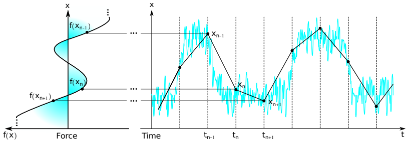
The central discovery is that the Gaussian prior is conjugate to the Gaussian thermal kicks in the overdamped Langevin equation, so after marginalizing the force values at the data points, the predictive distribution for the force at any chosen test points is a multivariate Gaussian. Its mean is $\tilde{\mu} = \zeta K_*^T (K + (2\zeta kT/\tau) I)^{-1} v$ and its covariance is $\tilde{K} = K_{**} - K_*^T (K + (2\zeta kT/\tau) I)^{-1} K_*$ (Eqs. 12–13). This turns force inference into a matrix-algebraic operation with no arbitrary discretization choice, and the same machinery supplies the conditional needed to Gibbs-sample the friction coefficient. The paper demonstrates on synthetic data from harmonic, quartic, and multi-well potentials that the method recovers the ground truth force with fewer data than the binned Masson et al. method or the residence-time histogram analysis do.

Load-bearing premise

The inference assumes the recorded positions are exact samples of an overdamped Langevin process with a single constant friction coefficient, and that the Euler time step is small enough that the discretized likelihood is accurate; if measurement noise is sizable or the sampling interval is too coarse, the likelihood is misspecified and the inferred force and friction become biased.

Editorial extensions

If this is right

For a single unbinned time trace of positions, the method yields a continuous effective force estimate with pointwise credible intervals, including in regions where data are sparse.
The accuracy of the inferred force improves as the number of data points grows, and the method converges to the ground truth force with fewer data points than the binned comparison methods tested.
When the friction coefficient is unknown, the Gibbs sampler still recovers both $\zeta$ and the force, though the force estimate is less accurate than when $\zeta$ is fixed.
The stiffness parameter $h = \zeta/\tau$ controls the signal-to-noise ratio; the method performs better for small stiffness (large thermal kicks relative to friction), consistent with the Langevin equation's structure.
The approach avoids binning artifacts such as the underestimation of forces in steep potential regions that arises when averaging within spatial bins.

Reading between the lines

Editorial extensions of the paper, not claims the author makes directly.

Because the likelihood assumes noiseless observations, the largest practical risk is measurement noise; explicitly modeling a Gaussian observation error by learning hidden positions, as the paper suggests, would extend the method to experimental single-particle tracking where localization error is significant.
The closed-form predictive should make the method amenable to sparse or inducing-point GP approximations, which would address the cubic scaling that currently limits the method to about 50,000 points.
The same conjugacy structure could be extended to memory kernels or position-dependent friction by choosing appropriate kernels or by Gibbs-sampling additional hyperparameters, though these go beyond what the paper tests.
A direct comparison of posterior predictive error against the true force on simulated data with added measurement noise would quantify the breakdown of the noiseless assumption; the paper does not report such a test.

Share X Bluesky LinkedIn Reddit HN

Signed reviews

No signed human review yet.

Editorial analysis

A structured set of objections, weighed in public.

Desk editor's note, referee report, and a circularity audit.

Desk Editor's Note

read the letter

You should know two things about this paper. First, the central idea is simple and correct: under forward-Euler overdamped Langevin dynamics, each measured increment (x_{n+1}-x_n) is a noisy observation of the force at x_n, with noise variance 2ζkT/τ. So the GP posterior predictive is standard GP regression with a physics-derived noise model. Second, the paper has a real derivation typo in the epsilon limit that is confusing but does not invalidate the final formulas.

What's actually new: applying Gaussian processes to force inference from single-particle or MD time traces, with a Gibbs sampler that draws both the force profile and the friction coefficient. The novelty is modest—this is a direct application of GP regression—but the packaging is useful. The synthetic tests are sensible: harmonic and multi-well potentials, convergence with N, and comparisons to Masson et al.'s binning and residence-time methods. The comparisons show the expected advantage of bin-free inference, especially in undersampled regions.

Soft spots, in proportion. The derivation of Eq. (10) as printed is internally inconsistent: adding εI to the test-point blocks of the augmented likelihood and taking ε→0 would pin f* to zero, not produce the stated posterior. The correct limit is zero precision on the test points (equivalently ε→∞ in their notation), and then the standard GP formulas follow. So the final expressions are right, but the presentation needs fixing.

The larger assumption is the Euler-discretized, noiseless likelihood. The paper explicitly states that it does not include observation noise and proposes an HMM extension in the Discussion, but it never tests how the method degrades when localization noise is comparable to thermal kicks or when τ is too large for Euler-Maruyama. For real single-molecule data this matters. It does not sink the paper, but it should be flagged more prominently and tested.

Two smaller issues: hyperparameters are hand-set (and in the multi-well example, the length scale was chosen with knowledge of the target's fine detail), and no code or data are provided, which limits reproducibility. The citation pattern is mostly fair—Masson et al. and residence time are the right baselines—though ref 37 is cited only for an analogy and never compared, so the 'first time' claim is not fully checked against it.

Verdict: the central claim—bin-free force inference with credible intervals from a Langevin trace—holds up under the stated assumptions. The paper is a solid methods contribution for single-molecule and coarse-grained MD analysis, not a conceptual breakthrough. A serious referee should look at it; I'd accept it into review and ask for a corrected derivation, a robustness check on observation noise, and preferably code. For a reading group, it's a decent example of GP inference in physics, but not a must-read.

Referee Report

3 major / 6 minor

Summary. The paper proposes a Bayesian nonparametric method for inferring an effective force f(x) from a time trace of positions generated by an overdamped Langevin dynamics. The force is assigned a zero-mean Gaussian process prior with a squared-exponential kernel, and the Euler-discretized dynamics provide a Gaussian likelihood for the increments. Combining prior and likelihood yields a Gaussian posterior for the force at arbitrary test points, with predictive mean and covariance given in Eqs. (12)-(13). The friction coefficient ζ is inferred jointly by a Gibbs sampler that alternately updates the force and ζ. The method is demonstrated on synthetic harmonic, multi-well, and quartic potentials, and is compared to the binning method of Masson et al. and to residence-time analysis, with the claim that it converges with fewer data points, provides full credible intervals, and avoids binning artifacts.

Significance. If the claims hold, the method is a useful addition to the analysis toolbox for single-molecule and molecular-dynamics trajectories, removing binning artifacts and providing pointwise uncertainties. The final predictive formulas are the standard Gaussian-process regression results, and the synthetic demonstrations are plausible. However, the derivation as written is incorrect, and the method is validated only on data generated from the same discretized model used in the likelihood; the advertised experimental applicability is therefore not yet supported. With corrected derivations and additional robustness experiments, the paper could be a solid methods contribution.

major comments (3)

[GP prior and posterior for force (Eqs. 8-13)] The derivation of the posterior predictive distribution is not valid. Eq. (9) is not an equivalent rewriting of Eq. (5): the likelihood P(x2:N|f(·),ζ,x1) does not involve the test-point values f*, and inserting f* with a degenerate variance εI does not create a likelihood for f*. Taking ε→0 forces f* to zero in the joint Gaussian, rather than producing a predictive distribution. Moreover, the marginal of the Gaussian in Eq. (10) over f* is N(0,K**), not Eq. (11). The correct route is to treat y_n = ζv_n as noisy observations of f(x_n) with noise variance 2ζkT/τ; the standard conditional Gaussian formulas then give exactly Eqs. (12)-(13) as the posterior mean and covariance of f* given the data. Please replace the erroneous epsilon-limit and marginalization argument with this (or an equivalent correct) derivation.
[Results and Discussion (noiseless Euler model)] The method is tested only on synthetic traces generated by the same Euler-discretized forward model that defines the likelihood, Eqs. (2)-(4). Since the Abstract and Introduction claim applicability to experimental traces, the manuscript should analyze or at least quantify the two main misspecifications: (i) localization/observation noise, under which consecutive increments become correlated and the diagonal likelihood is misspecified; and (ii) finite step size τ, where the Euler transition density deviates from the true transition density when the force varies appreciably over a diffusive step. Please add numerical experiments that measure bias and credible-interval coverage under these misspecifications, or explicitly restrict the experimental-applicability claims to the noiseless, small-τ regime and state this limitation in the abstract and conclusions.
[Gibbs sampling for friction coefficient] The Gibbs sampler is described only schematically, which prevents reproduction and assessment of the simultaneous inference claim. The Metropolis-Hastings update for ζ is not specified (proposal distribution, step size, tuning), and the paper does not state the number of iterations, burn-in, thinning, or the criterion used to select the MAP pair from the sampled sequence. To support Fig. 6 and the reported value ζ = 101.03 pg/µs, please provide these details and include convergence diagnostics or acceptance rates.

minor comments (6)

[SI, Hyperparameters; Fig. 9 caption] The notation for the hyperparameter sweep is confusing: 'σ = 10 in the figure corresponds to σ = 10ατ(vmax−vmin)' mixes the dimensionless figure label with the physical value. Please clarify the exact mapping used.
[SI, Eq. (26)] In Eq. (26), the kernel is defined as K(x,x′) but the right-hand side uses subscripts i and j (xi and x*j). Please correct the index notation to use x and x′.
[Fig. 5 and text on stiffness] The stiffness h = ζ/τ is labeled with units 'pg/µs' in Fig. 5, but from Eq. (15) h has units of pg/(µs·µs) if ζ is in pg/µs and τ in µs. Please correct the units in the figure and text.
[Gibbs sampling section] The statement 'After many iterations the sampled pairs converge to the true value' is imprecise: Gibbs sampling converges to the posterior distribution, not to a single true value; the MAP estimate is then extracted from the samples. Please rephrase.
[Reference [37]] Reference [37] (Frishman and Ronceray, 2018) is incomplete: it lacks a title and a journal, book, or arXiv identifier. Please complete the citation.
[Introduction] The claim 'So far no method satisfies all three criteria' is strong and is supported only by comparison to two binning-based baselines. Please consider acknowledging other binning-free or GP-based approaches, or broaden the comparison to justify the claim.

Circularity Check

0 steps flagged · score 0.0 of 10

No structural circularity: the force posterior is standard GP regression from an explicit Langevin likelihood, with hand-set prior hyperparameters rather than fitted predictions.

full rationale

The derivation is self-contained and does not reduce to its own inputs. The likelihood in Eq. (4) is the forward-Euler discretization of the overdamped Langevin equation, Eq. (3), and Eq. (5) is only a multivariate Gaussian rewriting of that same likelihood. Combining this likelihood with the zero-mean GP prior of Eq. (7) is exactly standard Gaussian process regression, and the posterior predictive mean and covariance in Eqs. (12)-(13) are the textbook result for that combination. No fitted parameter is renamed as a prediction: the GP hyperparameters σ and ℓ are hand-set from data ranges in the demonstrations, and the SI explicitly studies sensitivity to their choice; the friction coefficient ζ is assigned a Gamma prior and sampled via Gibbs updates from Eq. (14), not obtained by fitting the force prediction. Self-citations appear only in contextual or background references and are not load-bearing in the derivation. The method is validated against external baselines (Masson et al. and residence time) on synthetic data. The main caveat is that both the synthetic data and the likelihood share the same Euler-discretized, noiseless model, so the validation does not test misspecification under observation noise or larger time steps; that is a robustness limitation, not a circularity.

Assumptions & free parameters 6 free parameters · 6 assumptions · 0 invented entities

The method's predictive formulas are standard GP regression; the only hand-set quantities are the GP hyperparameters and the Gamma prior. No new physical entities are introduced. The main ledger burden is that sigma and l are chosen with knowledge of the data range and, in the multiwell case, of the target's fine detail.

free parameters (6)

GP prefactor sigma = alpha tau (vmax - vmin) with alpha = 1 pN/nm
Hand-set from the data range; controls prior uncertainty and pull toward measurements; sensitivity shown in SI Fig. 9.
GP length scale l = (xmax - xmin)/2 for harmonic, (xmax - xmin)/10 for multiwell
Hand-set; controls smoothness; reduced for the multiwell case to capture fine detail, informed by the test potential.
alpha in sigma rule = 1 pN/nm
Hand-picked prefactor in the hyperparameter rule.
Gamma prior shape alpha_zeta = 1
Weakly informative shape for the friction coefficient prior.
Gamma prior scale beta_zeta = 1000 pg/microsecond
Chosen to allow a large range for friction sampling.
Masson et al. bin count S = 10, 20, 50, 100 in comparisons
Chosen by hand for the baseline comparison; affects the baseline accuracy and therefore the comparison claim.

assumptions (6)

domain assumption The data-generating process is overdamped Langevin dynamics with constant friction and white Gaussian thermal noise (Eq. 1).
The model assumes the true physical process matches this equation, including the fluctuation-dissipation relation.
domain assumption Observed positions are noiseless; observation error is much smaller than thermal kicks (Methods, Dynamics model).
The paper states this assumption explicitly but does not quantify a breakdown threshold.
domain assumption The forward Euler discretization (Eq. 2) is a valid approximation of the continuous dynamics at the sampling step tau.
The likelihood uses Euler-Maruyama increments; discretization bias is not analyzed or bounded.
ad hoc to paper A zero-mean Gaussian process with squared exponential kernel is an appropriate prior for the effective force (Eq. 6).
This smoothness prior is chosen for convenience; the 'minimally committal' claim is weakened by this choice.
domain assumption A Gamma prior on the friction coefficient zeta (Eq. 14).
Convenient weakly informative prior; the paper does not test sensitivity to alpha and beta.
domain assumption The initial position x1 is known exactly.
The likelihood conditions on x1; initial condition uncertainty is not modeled.

how reviews work

0 comments

Cite this review

Pith. "Pith review of Inferring effective forces for Langevin dynamics using Gaussian processes." pith.science (2026). https://pith.science/paper/J7DGT4OS

@misc{pith2026190810484,
  author       = {Pith},
  title        = {Pith review of: Inferring effective forces for Langevin dynamics using Gaussian processes},
  year         = {2026},
  howpublished = {\url{https://pith.science/paper/J7DGT4OS}},
  note         = {Machine review of arXiv:1908.10484}
}

read the original abstract

Effective forces -- derived from experimental or {\it in silico} molecular dynamics time traces -- are critical in developing reduced and computationally efficient descriptions of otherwise complex dynamical problems. Thus, designing methods to learn effective forces efficiently from time series data is important. Of equal importance is the fact that methods should be suitable in inferring forces for undersampled regions of the phase space where data are limited. Ideally, a method should {\it a priori} be minimally committal as to the shape of the effective force profile, exploit every data point without reducing data quality through any form of binning or pre-processing, and provide full credible intervals (error bars) about the prediction. So far no method satisfies all three criteria. Here we propose a generalization of the Gaussian process (GP), a key tool in Bayesian nonparametric inference and machine learning, to achieve this for the first time.

Figures

Figures reproduced from arXiv: 1908.10484 by the authors.

**Figure 1.** Illustration of the goal of the analysis presented. A scalar degree of freedom, x, such as a particle’s position or an intra-molecular distance, is measured at discrete time levels, tn. The measurements obtained, xn, in turn, are used to find an effective force f(x). Despite the discrete measurements, the effective force found is a continuous function over x and extends also over positions that may not necessarily c… view at source ↗

**Figure 2.** Testing our method on a harmonic potential. This plot shows the inference of an effective force (and resulting effective potential) from a simple one-dimensional harmonic well test case. (A) the ground truth potential and our estimate obtained by integrating the MAP effective force estimate, (B) the ground truth force and the GP inferred effective force with uncertainty. (C) the time trace on which inference was per… view at source ↗

**Figure 3.** Testing our method as a function of the number of data points available. Here we show the effective force inferred from trajectories simulated for a particle trapped in a one dimensional harmonic well with a different number of data points. (A) 100 data points. (B) 1000 data points. (C) 10000 data points. Parameters used are specified in the main body. 12 [PITH_FULL_IMAGE:figures/full_fig_p012_3.png] view at source ↗

Figures from the paper (8 more)

**Figure 4.** Figure 4: Testing our method on a more complex, multi-well, potentials. Here we show the effective force (and effective potential) inferred from the time trace of a particle diffusing within a multi-well potential. (A) we show the ground truth and inferred effective potential. (…

**Figure 5.** Figure 5: Testing our method for different stiffness. Here we show the effective force inferred from 1000 point trajectories simulated for particles trapped in a one dimensional harmonic well using different choices of stiffness. (A) Stiffness is h = 100 pg/µs. (B) Stiffness is …

**Figure 6.** Figure 6: Results of simultaneous force and friction coefficient determination using Gibbs sampling. This figure shows the inference of the force and friction coefficient using a Gibbs sampler. (A) A histogram of the sampled friction coefficients simulates the posterior on ζ. Th…

**Figure 7.** Figure 7: Comparison of our method with others. In this figure, we compare our method to other methods of inference on three different effective force fields. The top compares inferences on the simplest, harmonic, potential (A,B). The middle compares inference on a quartic pote…

**Figure 8.** Figure 8: Error versus data points. Here we compare the error of each method. Error was calculated by integrating the absolute value of the predicted effective force (A) or potential (B) subtracted from the ground truth force or potential over the range [−1 nm, 1 nm]. Different …

**Figure 9.** Figure 9: Varying the hyperparameters. This plot shows inference of the effective force from a 1000 point time trace for a simulated particle trapped in a one dimensional harmonic well using different choices of hyperparameters. The prefactor, σ is varied on the vertical axis an…

**Figure 10.** Figure 10: Length scale determines detail of prediction 1. This plot shows the learned force from a low detail force field for different length scales and data points. Here the rows show different number of data points used and the columns show the different length scale used. T…

**Figure 11.** Figure 11: Length scale determines detail of prediction 2. This plot shows the learned force from a high detail force field for different length scales and data points. Here the rows show different number of data points used and the columns show the different length scale used. …

Discussion (0). Continue with ORCID to comment.

Reference graph

Works this paper leans on

44 extracted references · 44 canonical work pages

[1]

M.; Tiwary, P

Lamim Ribeiro, J. M.; Tiwary, P. Journal of Chemical Theory and Computation 2019, 15, 708--719

work page 2019
[2]

Akimov, A. V. The Journal of Physical Chemistry Letters 2017, 8, 5190--5195, PMID: 28985075

work page 2017
[3]

J.; Press \' e , S

Sgouralis, I.; Whitmore, M.; Lapidus, L.; Comstock, M. J.; Press \' e , S. Journal of Chemical Physics 2018, 148

work page 2018
[4]

M.; Levitus, M.; Sivasankar, S.; Press \'e , S

Jazani, S.; Sgouralis, I.; Shafraz, O. M.; Levitus, M.; Sivasankar, S.; Press \'e , S. Nature communications 2019, 10

work page 2019
[5]

Fundamentals of Statistical and Thermal Physics; Waveland Press, 2009

Reif, F. Fundamentals of Statistical and Thermal Physics; Waveland Press, 2009

work page 2009
[6]

Molecular Modeling and Simulation: An Interdisciplinary Guide; Springer-Verlag: Berlin, Heidelberg, 2002

Schlick, T. Molecular Modeling and Simulation: An Interdisciplinary Guide; Springer-Verlag: Berlin, Heidelberg, 2002

work page 2002
[7]

Nonequilibrium Statistical Mechanics; Oxford University Press, 2001

Zwanzig, R. Nonequilibrium Statistical Mechanics; Oxford University Press, 2001

work page 2001
[8]

Manzo, C.; Garcia-Parajo, M. F. Reports on Progress in Physics 2015, 78

work page 2015

Show all 44 references

[9]

Methods in Enzymology, 1st ed.; Elsevier Inc., 2012; Vol

Meijering, E.; Dzyubachyk, O.; Smal, I. Methods in Enzymology, 1st ed.; Elsevier Inc., 2012; Vol. 504; pp 183--200

2012
[10]

Biophysical Journal 2017, 112, 2021--2029

Sgouralis, I.; Press \' e , S. Biophysical Journal 2017, 112, 2021--2029

2017
[11]

Biophysical journal 2017, 112, 2117--2126

Sgouralis, I.; Press \'e , S. Biophysical journal 2017, 112, 2117--2126

2017
[12]

L.; Marqusee, S.; Bustamante, C.; Dill, K

Press \' e , S.; Peterson, J.; Lee, J.; Elms, P.; Maccallum, J. L.; Marqusee, S.; Bustamante, C.; Dill, K. Journal of Physical Chemistry B 2014, 118, 6597--6603

2014
[13]

Press \' e , S.; Lee, J.; Dill, K. A. Journal of Physical Chemistry B 2013, 117, 495--502

2013
[14]

Biophysical Journal 1993, 65, 2021--2040

Kusumi, A.; Sako, Y.; Yamamoto, M. Biophysical Journal 1993, 65, 2021--2040

1993
[15]

D.; Jacobson, K

Simson, R.; Sheets, E. D.; Jacobson, K. Biophysical Journal 1995, 69, 989--993

1995
[16]

Faraday Discussions 2015, 184, 359--379

Welsher, K.; Yang, H. Faraday Discussions 2015, 184, 359--379

2015
[17]

2018, 38--43

Wang, J.; Wehmeyer, C.; Noe', F.; Clementi, C. 2018, 38--43

2018
[18]

Poltavsky, I.; Sch, K. T. 2017, 1--6

2017
[19]

M.; Bouzida, D.; Swendsen, R

Kumar, S.; Rosenberg, J. M.; Bouzida, D.; Swendsen, R. H.; Kollman, P. A. Journal of Computational Chemistry 1992, 13, 1011--1021

1992
[20]

T.; Shell, M

Foley, T. T.; Shell, M. S.; Noid, W. G. Journal of Chemical Physics 2015, 143

2015
[21]

Izvekov, S.; Voth, G. A. Journal of Physical Chemistry B 2005, 109, 2469--2473

2005
[22]

J.; Risselada, H

Marrink, S. J.; Risselada, H. J.; Yefimov, S.; Tieleman, D. P.; De Vries , A. H. Journal of Physical Chemistry B 2007, 111, 7812--7824

2007
[23]

T \" u rkcan, S.; Alexandrou, A.; Masson, J. B. Biophysical Journal 2012, 102, 2288--2298

2012
[24]

B.; Casanova, D.; T \" u rkcan, S.; Voisinne, G.; Popoff, M

Masson, J. B.; Casanova, D.; T \" u rkcan, S.; Voisinne, G.; Popoff, M. R.; Vergassola, M.; Alexandrou, A. Physical Review Letters 2009, 102, 1--4

2009
[25]

Chemical Reviews 2017, 117, 7276--7330

Lee, A.; Tsekouras, K.; Calderon, C.; Bustamante, C.; Press \' e , S. Chemical Reviews 2017, 117, 7276--7330

2017
[26]

E.; Williams, C

Rasmussen, C. E.; Williams, C. K. I. Gaussian Processes for Machine Learning (Adaptive Computation and Machine Learning); The MIT Press, 2005

2005
[27]

Bayesian Data Analysis, Third Edition; Chapman & Hall/CRC Texts in Statistical Science; Taylor & Francis, 2013

Gelman, A.; Carlin, J.; Stern, H.; Dunson, D.; Vehtari, A.; Rubin, D. Bayesian Data Analysis, Third Edition; Chapman & Hall/CRC Texts in Statistical Science; Taylor & Francis, 2013

2013
[28]

von Toussaint, U. Rev. Mod. Phys. 2011, 83, 943--999

2011
[29]

N.; Li, C

Tavakoli, M.; Taylor, J. N.; Li, C. B.; Komatsuzaki, T.; Press \' e , S. Advances in Chemical Physics 2017, 162, 205--305

2017
[30]

Abraham, E

M.J. Abraham, E. L. B. H., D. van der Spoel; the GROMACS development team, GROMACS User Manual version 2019. http://www.gromacs.org

2019
[31]

LeVeque, R. Finite Difference Methods for Ordinary and Partial Differential Equations: Steady-State and Time-Dependent Problems (Classics in Applied Mathematics Classics in Applied Mathemat); Society for Industrial and Applied Mathematics: Philadelphia, PA, USA, 2007

2007
[32]

B.; Pedersen, M

Petersen, K. B.; Pedersen, M. S. The Matrix Cookbook; Technical University of Denmark, 2012; Version 20121115

2012
[33]

Bishop, C. M. Pattern Recognition and Machine Learning (Information Science and Statistics); Springer-Verlag: Berlin, Heidelberg, 2006

2006
[34]

Do, C. B. 2007, 1--13

2007
[35]

R.; Best, N

Gilks, W. R.; Best, N. G.; Tan, K. K. C. Journal of the Royal Statistical Society: Series C (Applied Statistics) 1995, 44, 455--472

1995
[36]

P.; Casella, G

Robert, C. P.; Casella, G. Monte Carlo Statistical Methods (Springer Texts in Statistics); Springer-Verlag: Berlin, Heidelberg, 2005

2005
[37]

Frishman, A.; Ronceray, P. 2018,

2018
[38]

L.; Pralle, A.; Stelzer, E

Florin, E. L.; Pralle, A.; Stelzer, E. H. K.; H \" o rber, J. K. H. Applied Physics A: Materials Science and Processing 1998, 66, 75--78

1998
[39]

Bayesian Anal

Nemeth, C.; Sherlock, C. Bayesian Anal. 2018, 13, 507--530

2018
[40]

K.; Rattray, M.; Lawrence, N

Titsias, M. K.; Rattray, M.; Lawrence, N. D. Bayesian Time Series Models 2011, 9780521196765, 295--316

2011
[41]

R.; Juang, B.-H

Rabiner, L. R.; Juang, B.-H. ASSP Magazine, IEEE 1986, 3, 4--16

1986
[42]

Rabiner, L. R. In Readings in Speech Recognition; Waibel, A., Lee, K.-F., Eds.; Morgan Kaufmann Publishers Inc.: San Francisco, CA, USA, 1990; Chapter A Tutorial on Hidden Markov Models and Selected Applications in Speech Recognition, pp 267--296

1990
[43]

Satija, R.; Das, A.; Makarov, D. E. Journal of Chemical Physics 2017, 147

2017
[44]

K. B. Petersen and M. S. Pedersen

Sgouralis, I.; Madaan, S.; Djutanta, F.; Kha, R.; Hariadi, R. F.; Press \' e , S. Journal of Physical Chemistry B 2019, 123, 675--688 mcitethebibliography main.bib0000664000000000000000000016500413531325265011173 0ustar rootroot @incollection Rabiner, author = Rabiner, Lawrenc...

2019

Pith tools

Reviewed August 14, 2026 · model on record in the stance chip above.

[1] [1]

M.; Tiwary, P

Lamim Ribeiro, J. M.; Tiwary, P. Journal of Chemical Theory and Computation 2019, 15, 708--719

work page 2019

[2] [2]

Akimov, A. V. The Journal of Physical Chemistry Letters 2017, 8, 5190--5195, PMID: 28985075

work page 2017

[3] [3]

J.; Press \' e , S

Sgouralis, I.; Whitmore, M.; Lapidus, L.; Comstock, M. J.; Press \' e , S. Journal of Chemical Physics 2018, 148

work page 2018

[4] [4]

M.; Levitus, M.; Sivasankar, S.; Press \'e , S

Jazani, S.; Sgouralis, I.; Shafraz, O. M.; Levitus, M.; Sivasankar, S.; Press \'e , S. Nature communications 2019, 10

work page 2019

[5] [5]

Fundamentals of Statistical and Thermal Physics; Waveland Press, 2009

Reif, F. Fundamentals of Statistical and Thermal Physics; Waveland Press, 2009

work page 2009

[6] [6]

Molecular Modeling and Simulation: An Interdisciplinary Guide; Springer-Verlag: Berlin, Heidelberg, 2002

Schlick, T. Molecular Modeling and Simulation: An Interdisciplinary Guide; Springer-Verlag: Berlin, Heidelberg, 2002

work page 2002

[7] [7]

Nonequilibrium Statistical Mechanics; Oxford University Press, 2001

Zwanzig, R. Nonequilibrium Statistical Mechanics; Oxford University Press, 2001

work page 2001

[8] [8]

Manzo, C.; Garcia-Parajo, M. F. Reports on Progress in Physics 2015, 78

work page 2015