REVIEW 3 major objections 5 minor 34 references
Gaussian Process modelling of granulation and oscillations in red-giant stars
T0 review · 3 major / 5 minor · reviewed 2026-08-14 · deepseek-v4-flash
Pith's one-line read Gaussian processes can pull red-giant oscillation parameters straight out of light curves.
desk verdict Solid, honest methods paper: the celerite-to-asteroseismic parameter mapping is genuinely new and nu_max recovery is robust, but the reported uncertainties need a calibration check before the precision claim is trusted. read the letter →
The pith
A machine-rendered reading of the paper's core claim, the machinery that carries it, and where it could break.
The reading
What carries the argument
The central object is the celerite SHOTerm kernel, a covariance function whose power spectral density is that of a stochastically driven, damped harmonic oscillator. At quality factor $Q=1/\sqrt{2}$ its PSD reduces to the Harvey-like form with an exponent of 4, the function usually used to model red-giant granulation in the frequency domain; for $Q>1$ the same kernel approximates the Gaussian-like shape of the oscillation bump. The model sums a granulation kernel (or two, in Model 2), an oscillation-bump kernel with $1.2<Q<18$, and a white-noise term. The kernel's hyperparameters $S_0$, $Q$, and $\omega_0$ are then mapped one-to-one onto the asteroseismic parameters $a_\mathrm{gran}$, $b_\mathrm{gran}$, $P_g$, and $\nu_\mathrm{max}$ via the normalization relations derived in Appendix A, so the GP fit returns physical stellar parameters rather than merely a flexible noise model.
What would settle it
Fit the same two-component kernel to high-cadence, high-signal-to-noise Kepler light curves of red giants whose granulation background has been independently measured, and compare the recovered $a_\mathrm{gran}$, $b_\mathrm{gran}$, and $\nu_\mathrm{max}$ against flexible power-spectrum fits; systematic discrepancies beyond the few-percent biases reported here, or failure to recover an injected Harvey component with a different slope (for example exponent 2 instead of 4), would invalidate the claimed parameter mapping.
Extended reading notes
Core claim
The paper's central claim is that a Gaussian-process model built from damped-harmonic-oscillator kernels can represent the photometric signal of a red-giant star, granulation plus the solar-like oscillation bump, directly in the time domain, and that the fitted kernel parameters can be translated into the same physical quantities normally extracted by power-spectrum fitting. The translation is carried out through the mapping $a_\mathrm{gran}=\sqrt{\sqrt{2}\, S_{0,\mathrm{gran}}\,\omega_{0,\mathrm{gran}}}$, $b_\mathrm{gran}=\omega_{0,\mathrm{gran}}/(2\pi)$, $P_g=4S_{0,\mathrm{bump}}Q^2$, and $\nu_\mathrm{max}=\omega_{0,\mathrm{bump}}/(2\pi)$. On TESS-like simulated light curves the model recovers $\nu_\mathrm{max}$ with about 1% bias and 3-4% scatter, and on 19 Kepler low-luminosity red giants the time-domain and power-spectrum determinations of $\nu_\mathrm{max}$ agree to within about 1-2%. The paper also reports a preliminary combined fit of the GP stellar model with a transit model that reduces the bias in $R_p/R_\star$ from 1.71% to -0.06% and the scatter from 6.49% to 5.80%. The authors note that a second granulation component's characteristic frequency is not constrained in the simulated data and that white noise is underestimated, which motivates their recommendation of the simpler one-granulation model for typical TESS time series.
Load-bearing premise
The argument depends on the assumption that the chosen kernel's power spectral density, a damped harmonic oscillator with quality factor fixed at $1/\sqrt{2}$ for granulation, matches the real granulation signal of red giants closely enough that the fitted kernel hyperparameters correspond one-to-one with the asteroseismic amplitudes, frequencies, and $\nu_\mathrm{max}$.
Editorial extensions
If this is right
- For 27.4-day TESS-like light curves of red giants, the simpler one-granulation model recovers $\nu_\mathrm{max}$ with roughly 1% bias and 3-4% scatter on simulated data, meaning asteroseismic characterization can be done in the time domain without building a full frequency-domain model.
- On real Kepler low-luminosity red giants, the time-domain GP and power-spectrum fits agree in $\nu_\mathrm{max}$ to within about 1-2%, indicating that the kernel choice does not introduce large systematic offsets in the main quantity of interest.
- Modelling the stellar GP simultaneously with a transit improves the estimated $R_p/R_\star$ from a 1.71% offset with 6.49% scatter to a -0.06% offset with 5.80% scatter in simulated injections, so evolved-host transit parameters benefit directly from treating stellar signals as correlated noise.
- Because the celerite kernels allow linear-scaling likelihood evaluation, the method can be applied to long TESS light curves, and the implementation is publicly available.
- The second granulation component's frequency is left unconstrained by TESS-like data, and white-noise levels are systematically underestimated in the two-component model, so the paper recommends Model 1 for typical TESS red-giant light curves.
Reading between the lines
- Editorial inference: if the same kernel mapping holds at longer baselines and higher signal-to-noise, GP-based time-domain analysis could take over the role of periodogram-based asteroseismic fitting for large red-giant samples, avoiding binning choices and providing a single model that also handles transits; this is a plausible extension, not a paper claim.
- Editorial inference: the cleanest test of the physical mapping is to let the granulation quality factor float in the fit; if the posterior converges near $Q=1/\sqrt{2}$ across many Kepler giants, the one-to-one calibration is confirmed, whereas systematic deviation would mean the reported $a_\mathrm{gran}$ and $b_\mathrm{gran}$ carry model-dependent bias. Such a test is not reported in the paper.
- Editorial inference: because the oscillation bump is treated as a single broad component, the recovered $\nu_\mathrm{max}$ describes the envelope rather than individual mode frequencies; combining this time-domain model with a mode-by-mode search could produce a pipeline that first extracts stellar parameters and then measures frequency spacings from the same framework.
Signed reviews
Editorial analysis
A structured set of objections, weighed in public.
Referee Report
Summary. The manuscript develops a Gaussian-process (GP) framework, built on the celerite package, to model granulation and oscillation signals in red-giant light curves directly in the time domain. Two models are considered: Model 1 uses one granulation kernel, an oscillation-bump kernel, and white noise; Model 2 adds a second granulation component. The method is applied to 20 TESS-like artificial low-luminosity red-giant stars and to 19 Kepler LLRGB stars, and the recovered parameters are compared with the injected values and with DIAMONDS power-spectrum fits. The paper reports a 1.14% bias and 3.34% scatter in nu_max on the simulated data, relative biases of 1.99% and 0.92% against DIAMONDS for Models 1 and 2, and a preliminary improvement in Rp/Rstar when the GP stellar model is fit jointly with a transit model. The authors are transparent about limitations: the second granulation frequency is unconstrained for every simulated star, white noise is underestimated in several configurations, and the GP and DIAMONDS uncertainties for nu_max sit below the paper's own stated lower bound from Eq. (13).
Significance. If the main result survives revision, the paper makes a useful contribution: it provides a publicly available and physically motivated celerite-kernel model for red-giant stellar signals, and the nu_max accuracy is supported by simulation and by agreement with an independent power-spectrum method. I give credit to the public implementation, the reproducible workflow, and the unusually clear reporting of unconstrained parameters. The method is of direct practical relevance for TESS light curves and for joint transit-and-stellar-noise modelling. However, the stated precision of the nu_max measurement is not yet established, because the GP credible intervals are smaller than the stated lower bound from Eq. (13) and no coverage test is presented. The transit result is explicitly preliminary but is advertised in the abstract, which raises the bar for documenting that experiment. With these caveats, the paper's significance is moderate rather than high: the core ideas are sound, but the central precision claim needs either empirical calibration or reformulation.
major comments (3)
- [Sec. 4.3, Eq. (13)] The paper's central claim that nu_max can be measured both accurately and precisely is not fully supported. The authors call Eq. (13) a lower limit for the uncertainty in nu_max, yet report <sigma_GP> = 3.43 microHz and <sigma_DIAMONDS> = 1.91 microHz against <sigma_nu_max> = 7.15 microHz. The subsequent appeal to DIAMONDS' successful literature applications cannot validate the GP HPD intervals, since it provides no direct test of whether the 68.3% GP intervals contain the true nu_max in the simulations or in injected signals. I request either a coverage test on the TESS-like simulations with the empirical coverage probability reported, or a reformulation of the abstract and conclusions that claims accuracy only and presents the GP uncertainties as model-based estimates that may be underestimated. This matters for downstream uses of the quoted uncertainties, such as scaling relations or ensemble asteroseismology.
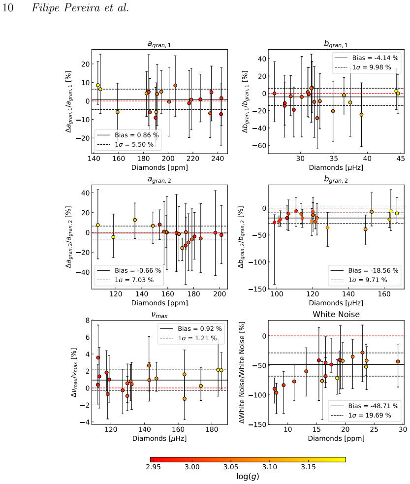
- [Sec. 3.2, Figs. 2-3] The simulation validation is partially internal, because the artificial light curves are generated using the same Kallinger et al. (2014) Harvey-like granulation functional form that defines the GP kernel through Eqs. (9)-(12). The paper's own results show the limits of this mapping: the second granulation frequency b_gran,2 is unconstrained for every simulated star, b_gran,1 is recovered with a 8.05% bias in Model 1, and white noise is systematically underestimated in Model 2. Consequently, the claim of recovering physically meaningful parameters is convincingly established only for nu_max; it is not established for the individual granulation parameters. I request either a simulation test using a different background shape (e.g., a different exponent or an additional background component) or a revised conclusion that limits the physical-parameter claim to nu_max and the oscillation envelope.
- [Sec. 5, Fig. 10] The transit experiment is presented as a partial validation of the abstract's claim about improving Rp/Rstar, but the manuscript does not state the number of injected transits, the orbital periods or depths, the limb-darkening model, or the SDE threshold used for detection. Without these details the comparison in Fig. 10 cannot be reproduced or evaluated. If the transit claim is retained in the abstract, the experimental setup should be documented; alternatively, the sentence should be removed or moved to the context of future work.
minor comments (5)
- [Sec. 4.2, Fig. 7] The text reports a relative white-noise bias of -48.71% with 16.89% scatter for Model 2, while the inset in Fig. 7 shows 1 sigma = 19.69%; this discrepancy should be reconciled.
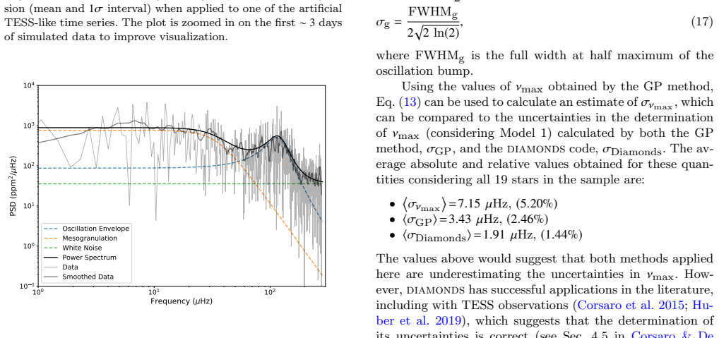
- [Eq. (13)] The printed form of Eq. (13) is typographically ambiguous: the expression '(1 + 4 (H_BR/sigma_g)^{2/3})' could be read as a sum rather than as the expected ratio formula from Kallinger et al. (2010). Please verify the formula and clarify whether it is a strict lower bound or an empirical expectation, since the text relies on that distinction.
- [Fig. 5 and Fig. 9] These figures show the PSD of the GP output and its components, but they do not overlay the input or DIAMONDS-comparable PSD model components; adding the true or reference background and oscillation envelope would help the reader judge how well the time-domain fit reproduces the frequency-domain structure.
- [Sec. 2.4] The authors correctly note that the Gelman-Rubin diagnostics are not strictly valid for correlated MCMC chains; however, the threshold of 1.1 and the practice of discarding up to 50% of each chain should be described with a reference or a brief justification, because these choices can affect the reported HPD intervals.
- [Fig. 10] The x-axis label 'Star' is uninformative; the figure would be clearer if the axis were labelled 'Star index (ordered by SDE)' and the SDE values were tabulated.
Circularity Check
No significant circularity: granulation recovery on synthetic data is self-consistent by construction, but the core nu_max claim rests on external Kepler/DIAMONDS comparison.
-
other
[Section 2.3 (Eqs. 8-9) and Section 3.1]
"To model the granulation power spectral density, a scaled version (to predict TESS granulation amplitudes) of model F of Kallinger et al. (2014) was adopted, which contains two granulation (or Harvey-like) components. ... Equation (9) has the same functional form as the equation commonly used to model the granulation in a power spectrum analysis (e.g., Kallinger et al. 2014). Since Eq. (9) corresponds to the PSD of the kernel in Eq. (8), this kernel can be used to capture the same granulation signal in the time domain."
The synthetic granulation time series used for validation are generated from the same Harvey-like functional form that the celerite SHOTerm kernel at Q = 1/sqrt(2) reproduces exactly. Therefore, the reported recovery of the granulation parameters agran and bgran from the simulated light curves is partly a self-consistency check of the kernel's assumed PSD shape rather than an independent test of the physical model. This does not compromise the paper's central claim about nu_max, because the oscillation signal in the simulations was injected via individual modes rather than with the GP bump kernel, and because the Kepler results are benchmarked against DIAMONDS, an independent power-spectrum fitting method.
full rationale
The paper's main derivation is a standard Bayesian GP parameter estimation: the kernel hyperparameters are mapped to asteroseismic parameters through the explicit, derived correspondences in Eqs. (9)-(12) and Appendix A, and no target quantity is fitted and then renamed as a prediction. The Kepler comparison against DIAMONDS is an external benchmark that does not depend on the GP assumptions, and the reported nu_max agreement (0.92-1.99% relative bias) supports the central claim independently of the synthetic simulations. The only partial circularity is that the TESS-like artificial granulation signal is generated with the same Harvey-like model family that the kernel assumes, so the granulation recovery on synthetic data is partly by construction; the paper itself acknowledges the resulting difficulties by finding that the second granulation frequency is unconstrained. This is a minor validation-design issue rather than a load-bearing circular derivation, and the self-citations in the paper (e.g., Campante et al. 2016, 2018) are used for noise models and scaling relations, not as an unverified uniqueness argument.
Assumptions & free parameters
free parameters (8)
- a_gran,1 (mesogranulation amplitude) =
per star, not tabulated; median over 5-10 subsets
- b_gran,1 (mesogranulation characteristic frequency) =
per star, not tabulated
- P_g (oscillation bump height) =
per star, not tabulated
- Q_bump =
per star, within [1.2, 18]
- nu_max =
per star; central result
- white noise =
per star, not tabulated
- a_gran,2 (granulation amplitude, Model 2) =
per star, not tabulated
- b_gran,2 (granulation frequency, Model 2) =
unconstrained for all simulated stars
assumptions (6)
- domain assumption Granulation power is described by a Harvey-like profile with exponent 4, as in Kallinger et al. (2014).
- domain assumption The oscillation power excess can be approximated by a celerite SHOTerm with Q > 1, whose PSD approximates the Gaussian-like oscillation bump.
- domain assumption The TESS photometric noise model from Sullivan et al. (2015) and Campante et al. (2016), plus a 20 ppm hr^(1/2) systematic term, describes real TESS noise.
- domain assumption Scaling relations for red-giant oscillations provide realistic input values for the simulated stars.
- domain assumption Non-overlapping 27.4-day subsets of a longer light curve are independent realizations of the stellar signal.
- domain assumption The celerite O(n) approximation, which restricts kernels to sums of exponentials or SHOTerms, is sufficient for red-giant granulation and oscillation signals.
Cite this review
Pith. "Pith review of Gaussian Process modelling of granulation and oscillations in red-giant stars." pith.science (2026). https://pith.science/paper/JXSU7MLH
@misc{pith2026190810662,
  author       = {Pith},
  title        = {Pith review of: Gaussian Process modelling of granulation and oscillations in red-giant stars},
  year         = {2026},
  howpublished = {\url{https://pith.science/paper/JXSU7MLH}},
  note         = {Machine review of arXiv:1908.10662}
}
abstract
The analysis of photometric time series in the context of transiting planet surveys suffers from the presence of stellar signals, often dubbed "stellar noise". These signals, caused by stellar oscillations and granulation, can usually be disregarded for main-sequence stars, as the stellar contributions average out when phase-folding the light curve. For evolved stars, however, the amplitudes of such signals are larger and the timescales similar to the transit duration of short-period planets, requiring that they be modeled alongside the transit. With the promise of TESS delivering on the order of $\sim\!10^5$ light curves for stars along the red-giant branch, there is a need for a method capable of describing the "stellar noise" while simultaneously modelling an exoplanet's transit. In this work, a Gaussian Process regression framework is used to model stellar light curves and the method validated by applying it to TESS-like artificial data. Furthermore, the method is used to characterize the stellar oscillations and granulation of a sample of well-studied \textit{Kepler} low-luminosity red-giant branch stars. The parameters determined are compared to equivalent ones obtained by modelling the power spectrum of the light curve. Results show that the method presented is capable of describing the stellar signals in the time domain and can also return an accurate and precise measurement of $\nu_\text{max}$, i.e., the frequency of maximum oscillation amplitude. Preliminary results show that using the method in transit modelling improves the precision and accuracy of the ratio between the planetary and stellar radius, $R_p/R_\star$. The method's implementation is publicly available.
Figures


Figures from the paper (6 more)




Reference graph
Works this paper leans on
-
[1]
Ambikasaran S., Foreman-Mackey D., Greengard L., Hogg D. W., O'Neil M., 2015, @doi [IEEE Transactions on Pattern Analysis and Machine Intelligence] 10.1109/TPAMI.2015.2448083 , http://adsabs.harvard.edu/abs/2015ITPAM..38..252A 38
arXiv 2015
-
[2]
Barclay T., Endl M., Huber D., Foreman-Mackey D., Cochran W. D., MacQueen P. J., Rowe J. F., Quintana E. V., 2015, @doi [ ] 10.1088/0004-637X/800/1/46 , http://adsabs.harvard.edu/abs/2015ApJ...800...46B 800, 46
-
[3]
M., Gully-Santiago M., Bryson S., Dotson J
Barentsen G., Hedges C., Saunders N., Cody A. M., Gully-Santiago M., Bryson S., Dotson J. L., 2018, preprint, https://ui.adsabs.harvard.edu/#abs/2018arXiv181012554B p. arXiv:1810.12554 ( @eprint arXiv 1810.12554 )
arXiv 2018
-
[4]
Brewer B. J., Stello D., 2009, @doi [ ] 10.1111/j.1365-2966.2009.14679.x , http://adsabs.harvard.edu/abs/2009MNRAS.395.2226B 395, 2226
arXiv 2009
-
[5]
Brooks S. P., Gelman A., 1998, @doi [Journal of Computational and Graphical Statistics] 10.1080/10618600.1998.10474787 , 7, 434
arXiv 1998
-
[6]
Campante T. L., et al., 2016, @doi [ ] 10.3847/0004-637X/830/2/138 , http://adsabs.harvard.edu/abs/2016ApJ...830..138C 830, 138
-
[7]
Synergy between asteroseismology and exoplanet science: an outlook
Campante T. L., Barros S. C. C., Demangeon O., da N \'o brega H. J., Kuszlewicz J. S., Pereira F., Chaplin W. J., Huber D., 2018, arXiv e-prints, https://ui.adsabs.harvard.edu/abs/2018arXiv181206150C p. arXiv:1812.06150
work page Pith review arXiv 2018
-
[8]
Carter J. A., Winn J. N., 2009, @doi [ ] 10.1088/0004-637X/704/1/51 , http://adsabs.harvard.edu/abs/2009ApJ...704...51C 704, 51
Show all 34 references
-
[9]
Corsaro E., De Ridder J., 2014, @doi [ ] 10.1051/0004-6361/201424181 , http://adsabs.harvard.edu/abs/2014A
2014 doi
-
[10]
A., 2015, @doi [ ] 10.1051/0004-6361/201525895 , http://adsabs.harvard.edu/abs/2015A
Corsaro E., De Ridder J., Garc \' a R. A., 2015, @doi [ ] 10.1051/0004-6361/201525895 , http://adsabs.harvard.edu/abs/2015A
2015 doi
-
[11]
P., Haywood R
Faria J. P., Haywood R. D., Brewer B. J., Figueira P., Oshagh M., Santerne A., Santos N. C., 2016, @doi [ ] 10.1051/0004-6361/201527899 , https://ui.adsabs.harvard.edu/#abs/2016A&A...588A..31F 588, A31
2016 doi
-
[12]
M., et al., 2018, @doi [ ] 10.3847/2041-8213/aadfde , https://ui.adsabs.harvard.edu/#abs/2018ApJ...865L..20F 865, L20
Farr W. M., et al., 2018, @doi [ ] 10.3847/2041-8213/aadfde , https://ui.adsabs.harvard.edu/#abs/2018ApJ...865L..20F 865, L20
2018 doi
-
[13]
Foreman-Mackey D., Agol E., Ambikasaran S., Angus R., 2017, @doi [ ] 10.3847/1538-3881/aa9332 , http://adsabs.harvard.edu/abs/2017AJ....154..220F 154, 220
2017 doi
-
[14]
Oxford: Oxford University Press, pp 169--193
Geweke J., 1992, in Bayesian Statistics 4. Oxford: Oxford University Press, pp 169--193
1992
-
[15]
W., Guenther D
Gruberbauer M., Kallinger T., Weiss W. W., Guenther D. B., 2009, @doi [ ] 10.1051/0004-6361/200811203 , https://ui.adsabs.harvard.edu/abs/2009A&A...506.1043G 506, 1043
2009 doi
-
[16]
K., et al., 2016, @doi [ ] 10.3847/0004-6256/152/6/185 , http://adsabs.harvard.edu/abs/2016AJ....152..185G 152, 185
Grunblatt S. K., et al., 2016, @doi [ ] 10.3847/0004-6256/152/6/185 , http://adsabs.harvard.edu/abs/2016AJ....152..185G 152, 185
2016 doi
-
[17]
K., et al., 2017, @doi [ ] 10.3847/1538-3881/aa932d , http://adsabs.harvard.edu/abs/2017AJ....154..254G 154, 254
Grunblatt S. K., et al., 2017, @doi [ ] 10.3847/1538-3881/aa932d , http://adsabs.harvard.edu/abs/2017AJ....154..254G 154, 254
2017 doi
-
[18]
235, Future Missions in Solar, Heliospheric & Space Plasma Physics
Harvey J., 1985, in Rolfe E., Battrick B., eds, ESA Special Publication Vol. 235, Future Missions in Solar, Heliospheric & Space Plasma Physics
1985
-
[19]
D., et al., 2014, @doi [ ] 10.1093/mnras/stu1320 , https://ui.adsabs.harvard.edu/abs/2014MNRAS.443.2517H 443, 2517
Haywood R. D., et al., 2014, @doi [ ] 10.1093/mnras/stu1320 , https://ui.adsabs.harvard.edu/abs/2014MNRAS.443.2517H 443, 2517
2014 doi
-
[20]
X., et al., 2018, preprint, http://adsabs.harvard.edu/abs/2018arXiv180905967H ( @eprint arXiv 1809.05967 )
Huang C. X., et al., 2018, preprint, http://adsabs.harvard.edu/abs/2018arXiv180905967H ( @eprint arXiv 1809.05967 )
2018 arXiv
-
[21]
Huber D., et al., 2019, @doi [ ] 10.3847/1538-3881/ab1488 , https://ui.adsabs.harvard.edu/abs/2019AJ....157..245H 157, 245
2019 doi
-
[22]
Kallinger T., et al., 2010, @doi [ ] 10.1051/0004-6361/200811437 , https://ui.adsabs.harvard.edu/abs/2010A&A...509A..77K 509, A77
2010 doi
-
[23]
Kallinger T., et al., 2014, @doi [ ] 10.1051/0004-6361/201424313 , http://adsabs.harvard.edu/abs/2014A
2014 doi
-
[24]
A., Huber D., Matthews J
Kallinger T., Hekker S., Garcia R. A., Huber D., Matthews J. M., 2016, @doi [Science Advances] 10.1126/sciadv.1500654 , http://adsabs.harvard.edu/abs/2016SciA....2E0654K 2, 1500654
2016 doi
-
[25]
Kov \'a cs G., Zucker S., Mazeh T., 2002, @doi [ ] 10.1051/0004-6361:20020802 , http://adsabs.harvard.edu/abs/2002A
2002 doi
-
[26]
Kreidberg L., 2015, @doi [ ] 10.1086/683602 , http://adsabs.harvard.edu/abs/2015PASP..127.1161K 127, 1161
2015 doi
-
[27]
S., Chaplin W
Kuszlewicz J. S., Chaplin W. J., North T. S. H., Farr W. M., Bell K. J., Davies G. R., Campante T. L., Hekker S., 2019, @doi [ ] 10.1093/mnras/stz1689 , https://ui.adsabs.harvard.edu/abs/2019MNRAS.488..572K 488, 572
2019 doi
-
[28]
Mathur S., et al., 2011, @doi [ ] 10.1088/0004-637X/741/2/119 , http://adsabs.harvard.edu/abs/2011ApJ...741..119M 741, 119
2011 doi
-
[29]
Mosser B., et al., 2012, @doi [ ] 10.1051/0004-6361/201117352 , https://ui.adsabs.harvard.edu/abs/2012A&A...537A..30M 537, A30
2012 doi
-
[30]
North T. S. H., et al., 2017, @doi [ ] 10.1093/mnras/stw2782 , http://adsabs.harvard.edu/abs/2017MNRAS.465.1308N 465, 1308
2017 doi
-
[31]
Adaptive Computation and Machine Learning, MIT Press, Cambridge, MA, USA
Rasmussen C., Williams C., 2006, Gaussian Processes for Machine Learning. Adaptive Computation and Machine Learning, MIT Press, Cambridge, MA, USA
2006
-
[32]
R., et al., 2015, @doi [Journal of Astronomical Telescopes, Instruments, and Systems] 10.1117/1.JATIS.1.1.014003 , http://adsabs.harvard.edu/abs/2015JATIS...1a4003R 1, 014003
Ricker G. R., et al., 2015, @doi [Journal of Astronomical Telescopes, Instruments, and Systems] 10.1117/1.JATIS.1.1.014003 , http://adsabs.harvard.edu/abs/2015JATIS...1a4003R 1, 014003
2015 doi
-
[33]
W., et al., 2015, @doi [ ] 10.1088/0004-637X/809/1/77 , http://adsabs.harvard.edu/abs/2015ApJ...809...77S 809, 77
Sullivan P. W., et al., 2015, @doi [ ] 10.1088/0004-637X/809/1/77 , http://adsabs.harvard.edu/abs/2015ApJ...809...77S 809, 77
2015 doi
-
[34]
Vanderspek R., et al., 2018, preprint, http://adsabs.harvard.edu/abs/2018arXiv180907242V ( @eprint arXiv 1809.07242 )
2018 arXiv
Reviewed August 14, 2026 · model on record in the stance chip above.
Discussion (0). Continue with ORCID to comment.