Gradient-Based STL Control with Application to Nonholonomic Systems

Dimos V. Dimarogonas; Peter Varnai

REVIEW 3 major objections 6 minor 15 references

Gradient-Based STL Control with Application to Nonholonomic Systems

T0 review · 3 major / 6 minor · reviewed 2026-08-14 · deepseek-v4-flash

Challenge this review Re-run · record.json Download PDF Read on arXiv ↗ Review JSON

Pith's one-line read The paper claims that, for a class of unicycle-like systems, a temporal-logic task can be enforced by two stacked gradient controllers—one that keeps the task-robustness measure above a designed curve and one that keeps the…

desk verdict Useful unicycle extension of gradient-based STL control, but Theorem 3 as stated misses a C^2 requirement on rho_psi; fixable, worth refereeing. read the letter →

arxiv 1909.02483 v1 pith:TF7YAAKG submitted 2019-09-05 eess.SY cs.SY

Peter Varnai , Dimos V. Dimarogonas This is my paper · ORCID

classification eess.SYcs.SY

keywords signaltemporallogicgradient-basedcontrolprescribedperformancenonholonomicsystemsunicycledynamicsrobustnesssatisfactionbarrierfunctionstaskspecifications

verification ladder T0 review T1 audit T2 compute T3 formal

The pith

A machine-rendered reading of the paper's core claim, the machinery that carries it, and where it could break.

The reading

The paper turns a signal temporal logic (STL) task—such as 'reach a goal within ten seconds and then stay near it'—into feedback laws that only act when a robustness measure approaches a user-chosen lower curve. For simple dynamics a single controller keeps the measure above the curve and thereby guarantees the task, provided the system state remains bounded. The paper's main extension handles unicycle-like nonholonomic systems: a naive gradient controller fails because the direction in which it can push the robustness metric may vanish, so a second, auxiliary controller is added to keep that direction away from zero. The two controllers together give what the paper calls local robustness satisfaction, and the intention is to use such inexpensive controllers to guide exploration inside learning algorithms.

What carries the argument

The machinery is a Nagumo-type invariance argument over time-varying sets defined by the robustness measure. Each task is packaged as a region of interest $X(t)=\{x:\gamma(t)\le \rho_\psi(x)\le\Gamma(t)\}$ with $\Gamma(t)\ge\gamma(t)+\epsilon$, and the control is zero in the uncontrolled region $A(t)=\{\rho_\psi(x)>\Gamma(t)\}$, so the controller is active only when the measure is near its lower bound. On the boundary $\rho_\psi=\gamma(t)$, the control law (6), $u=\kappa(x,t)\frac{K v(x)}{\|v(x)\|_2^2+\Delta}$, is chosen so that $\dot{\rho}_\psi\ge\dot{\gamma}$, which by the generalized Nagumo theorem prevents the trajectory from crossing below the curve. For unicycle-like systems the same construction is applied to the augmented robustness $\rho_{\psi_{\mathrm{aug}}}=\|v(x)\|_2-v_{\min}$, with the second input acting through the coefficient $v_{\mathrm{aug}}(x)^T=\frac{v(x)^T}{\|v(x)\|_2}\frac{\partial v}{\partial x_2}g_{22}(x)$; Theorem 3 combines the two invariance conditions.

What would settle it

Simulate the unicycle system (9)-(10) with additive process noise, starting from an initial state inside the domain $D$ with $\rho_\psi(x_1(0))\ge\gamma(0)$ and $\rho_{\psi_{\mathrm{aug}}}(x(0))\ge\gamma_{\mathrm{aug}}(0)$, and apply (15)-(19). If along any such trajectory the solution exists beyond the claimed interval but either $\rho_\psi$ or $\rho_{\psi_{\mathrm{aug}}}$ falls below its curve before the state leaves $D$, then Theorem 3 is false. A direct check of the boundary condition $\dot{\rho}_\psi\ge\dot{\gamma}$ at $\rho_\psi=\gamma(t)$ with the formulas (15) and (19) would likewise settle the claim.

Watch

Extended reading notes

Core claim

The central claim is Theorem 3: for the triangular system (10), under Assumptions 1 and 3, the control laws (15) and (19) achieve local robustness satisfaction of the conjoined specification $\rho_\psi(x_1(t)) \ge \gamma(t)$ and $\rho_{\psi_{\mathrm{aug}}}(x(t)) \ge \gamma_{\mathrm{aug}}(t)$ within the domain $D$. Here $\rho_\psi$ is the spatial robustness of a non-temporal formula $\psi$, and $\gamma(t)$ is a designed curve whose domination by $\rho_\psi$ guarantees the temporal task $\varphi$ by Assumption 1(iii). Because a direct gradient step on $\rho_\psi$ may be impossible when the direction $v(x)^T = \frac{\partial \rho_\psi}{\partial x_1} g_{11}(x_2)$ vanishes, the paper defines an augmented task $\rho_{\psi_{\mathrm{aug}}}(x) = \|v(x)\|_2 - v_{\min}$ and uses the second input to keep $v$ bounded away from zero. Theorem 3 says these two invariance conditions hold together for finite time; if the state also remains bounded, Theorem 2 upgrades local robustness satisfaction to satisfaction of the original STL task.

Load-bearing premise

The guarantee only holds while the robot's heading is neither exactly perpendicular nor exactly parallel to the direction of the target error; at either of those two headings one of the two control directions vanishes, and the theorem's assumptions stop applying.

Editorial extensions

If this is right

For any system fitting the triangular form (10) and satisfying the two non-vanishing-direction assumptions, a temporal-logic task can be certified by two independent, minimally invasive feedback laws—one per input channel—that are active only near the robustness lower bound.
If the state remains bounded, or if the conjoined specifications themselves enforce boundedness, the local guarantee of Theorem 3 becomes global satisfaction of the STL task by Theorem 2.
A conjunction of several such tasks can be controlled by a weighted consensus (20) that gives priority to whichever robustness measure is closest to its lower bound; individual guarantees are traded for cheap, combined steering, which is the intended use in policy-improvement learning.
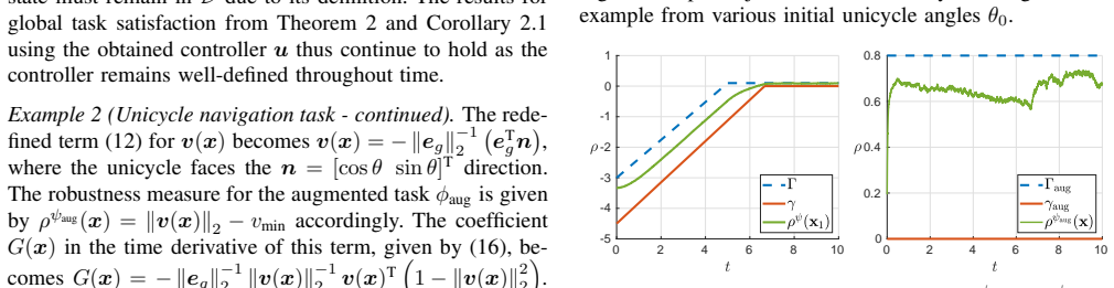
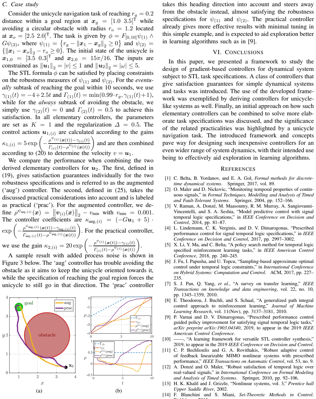
With a nonzero regularization parameter $\Delta>0$, the second input can influence the second derivative of the robustness metric; the paper's 'practical' controller (25) uses that mechanism to steer a unicycle away from an obstacle while still heading toward the goal.
Configurations where the controllability direction vanishes are outside the theorem: such states are excluded from the domain $D$ by the augmented task, so the guarantee is explicitly local and conditional.

Reading between the lines

Editorial extensions of the paper, not claims the author makes directly.

The authors leave implicit that the same augmented-task construction could extend inductively to systems with several nonholonomic constraints: after $v_1\neq 0$ is enforced, a second augmented task can enforce $v_2\neq 0$, and so on.
Not addressed in the paper is a wrapper controller that keeps the state inside $D$, or a mode-switching controller that first rotates the heading away from the excluded perpendicular and parallel configurations; such a wrapper would turn the local guarantee into a global one for unicycle tasks.
A tunable consequence not drawn by the paper is that the regularization parameter $\Delta$ could serve as an exploration knob in a learning loop, since larger $\Delta$ changes how strongly the steering input responds to the second derivative of robustness.
The case study suggests a testable extension: once exact guarantees are relaxed, steering by the second derivative (the 'practical' controller) may outperform maintaining the augmented invariant set, and a sweep over obstacle placements and initial headings would quantify the trade-off.

Share X Bluesky LinkedIn Reddit HN

Signed reviews

No signed human review yet.

Editorial analysis

A structured set of objections, weighed in public.

Desk editor's note, referee report, and a circularity audit.

Desk Editor's Note

read the letter

Colleague,

This paper is worth reading for the unicycle extension. The augmented task of keeping ||v|| away from zero is a neat idea that addresses a real failure mode of PPC-style controllers for nonholonomic systems. Theorem 1 also generalizes the prior PPC and barrier-function results by dropping concavity and full-row-rank assumptions, which is a modest but real contribution.

That said, the main theorem has a load-bearing gap that the stress-test note identifies correctly. Theorem 3 relies on Assumption 1(i), which only gives locally Lipschitz gradients of rho_psi. But the augmented controller (19) uses ∂v/∂x in (16)-(17), and v contains ∂rho_psi/∂x. That requires second derivatives. The concrete counterexample in the note works: rho_psi = x1|x1|/2 + x1 satisfies Assumption 1(i) but the augmented control is undefined at x1=0. So the statement of Theorem 3 is not true as written for all systems satisfying its assumptions. This is fixable by adding an explicit C^2 assumption on rho_psi and corresponding differentiability of g11; the proof structure then holds. It's a technical gap, not a conceptual disaster, but it should be fixed before the guarantees are used.

The non-degeneracy assumptions also exclude some practically relevant states. The paper acknowledges the perpendicular case is excluded from D and the parallel case by parameter choice, but there is no controller driving such states into D. That is a limitation worth stating explicitly.

The combination scheme in Section V is explicitly heuristic, and the case study is a single qualitative simulation. That is fine given the paper frames it as initial thoughts, but it shouldn't be overread.

The citations look appropriate, including the self-citations to the companion learning papers, since those are used for motivation rather than to claim novelty.

Overall, this is a solid, honest paper for the STL-control community. It deserves a serious referee; the smoothness gap is likely to be caught and fixed in revision. I would bring it to a reading group and would cite the unicycle extension after the C^2 fix lands.

Recommendation: send to peer review with a request for revision.

Referee Report

3 major / 6 minor

Summary. The paper proposes gradient-based controllers for signal temporal logic (STL) specifications. For systems of the form ẋ = f(x)+g(x)u+w, it defines a control law (Theorem 1) that guarantees local robustness satisfaction ρψ(x(t)) ≥ γ(t) by enforcing Nagumo-type boundary conditions, assuming the gradient of the robustness metric is controllable (Assumption 2). It then extends the approach to unicycle-like systems (10) by introducing an augmented robustness specification ρψ_aug = ||v(x)|| - v_min whose purpose is to keep the controllability term v(x) away from zero. The main theoretical result, Theorem 3, states that the two control laws (15) and (19) jointly achieve local robustness satisfaction of the conjoined specification within a domain D. The paper also discusses how elementary controllers can be combined (Section V) and illustrates the approach on a unicycle navigation example and a case study with obstacle avoidance.

Significance. If the technical gaps identified below are repaired, the paper offers a computationally inexpensive, local-satisfaction controller for a class of nonholonomic systems with STL tasks, complementing MPC and barrier-function approaches. The explicit construction of an augmented task to avoid singular controllability directions is a useful idea, and the paper is honest about the loss of guarantees when controllers are combined. The theoretical claims are, however, conditional on regularity assumptions that are not fully stated, so the main theorem as written is not established for the general system class claimed.

major comments (3)

[§IV, Lemma 5 (application of Lemma 3)] Assumption 1(i) only requires ρψ and its gradient to be locally Lipschitz, but the augmented controller (19) uses ∂v/∂x1 and ∂v/∂x2, i.e., second derivatives of ρψ. This is not implied by the stated assumption. For example, take x1,x2 ∈ R, dynamics ẋ1 = x2 u1, ẋ2 = u2, and ρψ(x1) = x1|x1|/2 + x1 with g11(x2)=x2. Then ∂ρψ/∂x1 = |x1|+1 is locally Lipschitz, so Assumption 1(i) is satisfied, but the second derivative is undefined at x1=0. With v(x) = (|x1|+1)x2, the point x0=(0,1) lies in the appropriate domain for suitable γ_aug, Γ_aug, and vmin, and vaug(x0) ≠ 0, yet ∂v/∂x1 does not exist at x0. Consequently, the κ_aug condition in Lemma 5 is not well-defined, u2 in (19) need not be locally Lipschitz, and Lemma 1 cannot be applied. The unicycle example is smooth away from eg = 0, so the simulations are unaffected, but Theorem 3 as stated for general system (10) requires an explicit C^2 assumption on ρψ (and corresponding differentiability of g11, g21, g22) that is absent from Assumption 1.
[§IV, Theorem 3 (proof)] The proof of Lemma 5 invokes Lemma 3 (Nagumo) for the time-varying set S_aug(t) = {x : γ_aug(t) − ρψ_aug(x) ≤ 0}. Lemma 3 requires ∂ζ/∂x ≠ 0 at the boundary, i.e., ∂ρψ_aug/∂x ≠ 0 on ∂X_aug. This is not established from Assumption 3. Assumption 3 only states that vaug(x) ≠ 0 in the augmented region of interest; it does not imply that the gradient of ρψ_aug is nonzero on the boundary. Without this condition, the invariance argument for the augmented specification is incomplete. Adding a C^2 regularity assumption would make ∂ρψ_aug/∂x well-defined, but nonvanishing still needs to be checked or imposed.
[§IV, Theorem 3 (proof)] The proof of Theorem 3 proceeds by taking δ = min(δ1, δ2) from Lemmas 4 and 5, but each lemma assumes that the other control input is already Lipschitz continuous. In the coupled closed loop, u1 and u2 are both determined by the same state, so one must verify that the joint right-hand side is locally Lipschitz before applying Lemma 1. This is a fixable issue once the missing C^2 assumption is added, but as written the existence argument for the combined system is not fully rigorous.

minor comments (6)

[Definition 1 and §IV (Eq. (14))] The phrasing 'ρψ(x) and its gradient ∂ρψ/∂x are locally Lipschitz continuous' is ambiguous; it should explicitly state that ρψ is C^1 with a locally Lipschitz gradient, or otherwise clarify the differentiability class.
[Assumption 2 and Assumption 3] The definition D := {x : ∃t, x ∈ (X(t) ∪ A(t)) ∩ (A_aug(t) ∪ X_aug(t))} uses an existential quantifier inside a set builder, which is confusing. It should be written as a union over t, and the subsequent condition (14) should be stated for all x ∈ D, not with an additional '∃t' quantifier.
[Theorem 1 and Lemma 4 proofs] The quantifier structure in (5) and (18), 'v(x) ≠ 0, ∀x : ∃t s.t. x ∈ X(t)', is nonstandard. It should be 'for all x and all t such that x ∈ X(t), v(x) ≠ 0' to be unambiguous.
[Definition 1] In the proofs, the noise bound uses 'max_w' without specifying the set B over which w ranges; this should be defined explicitly, e.g., as a supremum over the bounded set B.
[Example 2 and Section V-C] The notation for the upper boundary ¯X(t) and lower boundary ¯X(t) appears identical in the typeset version; the authors should use visually distinct symbols (e.g., overbar and underline) to avoid confusion.
[Example 2 and Section V-C] The paper should state clearly that the main guarantee requires the initial state to satisfy ρψ_aug(x(0)) ≥ γ_aug(0); if the system starts at a configuration where v = 0 or vaug = 0, the controller (19) is not well-defined and the theorem does not apply. This limitation is acknowledged in Example 2 but should appear as a remark after Theorem 3.

Circularity Check

0 steps flagged · score 0.0 of 10

No circularity: the main theorems are conditional guarantees proved from stated assumptions with design parameters, and the self-citations are only motivational.

full rationale

The derivation chain is self-contained. Section III defines the robustness measure and states Assumption 1; Theorem 1 proves that the chosen feedback u(x,t) with κ chosen at the boundary dominates the dynamics and noise terms and yields the Nagumo condition ρ̇_ψ ≥ γ̇, with K and Δ being free design parameters, not fitted quantities. Theorem 2 is a direct consequence of Lemma 2 once boundedness is assumed. In Section IV, the unicycle extension explicitly derives v(x), introduces the augmented task ψ_aug with ρ_ψ_aug = ‖v‖ − v_min, and states Assumption 3 as a controllability condition; Lemmas 4 and 5 prove local robustness satisfaction for u1 and u2 under the stated hypotheses, and Theorem 3 composes these lemmas. All claims are conditional on Assumptions 1 and 3 and on the well-posedness of the control laws; no quantity is fitted from data and then called a prediction. The self-citations [9] and [10] appear only in the introduction and conclusion to motivate the exploration-aiding use of such controllers; they do not enter the proof chain and are not load-bearing. A separate correctness question about whether ∂v/∂x exists under Assumption 1(i) in equations (16)–(17) is a regularity gap, not an instance of circularity.

Assumptions & free parameters 5 free parameters · 6 assumptions · 1 invented entities

The central claim rests on the standard existence and invariance theorems, on the explicitly stated Assumptions 1-3, and on an unstated C^2 / d v smoothness requirement. The main design parameters are the gain constants and specification curves, which are user choices rather than fitted data. No new physical entities are postulated; the only new mathematical device is the augmented non-degeneracy task, whose feasibility is an added assumption.

free parameters (5)

K and Delta (regularization gains) = K = 1, Delta = 0.5 in the case study
Controller parameters appear in equations (6), (15), and (19); proofs require (K - 1) v_min^2 >= Delta. They are design choices, not fitted to data, but they shape the closed-loop behavior.
v_min (augmented margin) = 0.001 in the case study
Defines the augmented task rho_psi_aug = ||v|| - v_min and the domain D. Too large a margin can exclude feasible unicycle trajectories, and the theorem requires the augmented task to be initially satisfied.
Specification curves gamma(t) and Gamma(t) = gamma(1) = -4 + 2.5t, Gamma(1) = min(0.99*rg, gamma(1) + 1); gamma(2) = 0, Gamma(2) = 0.5 in the case study
These curves encode the task and define the region of interest; Assumption 1(iii)-(iv) requires them to be feasible from the initial state. They are user choices per task, not fitted constants.
Gain scale constants in kappa = 2 in Example 2; 5, 5, and 20 in the case study
The kappa functions use exponential forms with hand-picked constants. The theorems only require kappa to dominate the dynamics bounds at the lower boundary, and the chosen values in simulation are convenient choices, not derived from the dynamics.
Combination weights alpha(i) = alpha(i) = (Gamma(i) - rho_psi_i) / (Gamma(i) - gamma(i)) if rho <= Gamma, else 0
Used in the heuristic combination equation (20) to prioritize the most violated specification; no guarantee accompanies this choice.

assumptions (6)

domain assumption Local Lipschitz continuity of f, g, rho_psi and its gradient, and piecewise continuous bounded noise w, plus existence of a feasible curve gamma(t) with rho_psi(x0) >= gamma(0) (Assumption 1)
Used throughout Sections III and IV to apply existence, uniqueness, and invariance theorems.
domain assumption v(x) = d(rho_psi)/dx1 * g11(x2) is nonzero for states in X(t) (Assumption 2, equation (5))
Necessary for u1 to be Lipschitz and able to increase rho_psi near the lower boundary; fails for a unicycle perpendicular to the target.
domain assumption v_aug(x) is nonzero for states in X_aug(t) (Assumption 3, equation (18))
Necessary for u2 to regulate the augmented task; fails when the unicycle heading is parallel to the target error.
ad hoc to paper The augmented controller requires d v / d x, hence second derivatives of rho_psi, to exist and be locally Lipschitz; this is not stated in Assumption 1
Equations (16)-(17) and Lemma 5 differentiate v(x), which only has a Lipschitz gradient under Assumption 1. The paper does not flag this extra smoothness requirement.
standard math Standard existence, uniqueness, and generalized Nagumo invariance theorems (Lemmas 1-3 from Khalil and Blanchini)
Used to prove local existence and forward invariance of the set rho_psi >= gamma.
domain assumption The state remains bounded under the locally robustness satisfying control law, as required by Theorem 2 for global STL satisfaction
The paper notes this can be viewed as an added task specification; it is not guaranteed by the controller alone.

invented entities (1)

Augmented task rho_psi_aug(x) = ||v(x)|| - v_min
purpose: Keeps v(x) nonzero in the region of interest so that the primary controller u1 remains well-defined and effective
Auxiliary mathematical specification introduced by the authors; it has no external falsifiable handle and its feasibility restricts the set of initial states.

how reviews work

0 comments

Cite this review

Pith. "Pith review of Gradient-Based STL Control with Application to Nonholonomic Systems." pith.science (2026). https://pith.science/paper/TF7YAAKG

@misc{pith2026190902483,
  author       = {Pith},
  title        = {Pith review of: Gradient-Based STL Control with Application to Nonholonomic Systems},
  year         = {2026},
  howpublished = {\url{https://pith.science/paper/TF7YAAKG}},
  note         = {Machine review of arXiv:1909.02483}
}

read the original abstract

In this paper, we study the control of dynamical systems under temporal logic task specifications using gradient-based methods relying on quantitative measures that express the extent to which the tasks are satisfied. A class of controllers capable of providing satisfaction guarantees for simple systems and specifications is introduced and then extended for the case of unicycle-like dynamics. The possibility of combining such controllers in order to tackle more complex task specifications while retaining their computational efficiency is examined, and the practicalities related to an effective combination are demonstrated through a simulation study. The introduced framework for controller design lays ground for future work in the direction of effectively combining such elementary controllers for the purpose of aiding exploration in learning algorithms.

Figures

Figures reproduced from arXiv: 1909.02483 by the authors.

**Figure 2.** Evolution of robustness measures ρ ψ and ρ ψaug for the unicycle example in the sample case θ0 = 11π/16. V. COMBINING CONTROLLERS In this section, we examine the possibility and practicalities associated with using the derived controllers in combination with one another in order to extend the range of STL task specifications we can satisfy. The motivation behind this is that controllers for a single robustness spe… view at source ↗

**Figure 3.** (a) Sample trajectories and (b) evolution of robustn [PITH_FULL_IMAGE:figures/full_fig_p008_3.png] view at source ↗

Discussion (0). Continue with ORCID to comment.

Reference graph

Works this paper leans on

15 extracted references · 15 canonical work pages

[1]

Belta, B

C. Belta, B. Y ordanov, and E. A. Gol, F ormal methods for discrete- time dynamical systems . Springer, 2017, vol. 89

work page 2017
[2]

Monitoring temporal properti es of contin- uous signals,

O. Maler and D. Nickovic, “Monitoring temporal properti es of contin- uous signals,” in F ormal Techniques, Modelling and Analysis of Timed and Fault-Tolerant Systems . Springer, 2004, pp. 152–166

work page 2004
[3]

Model predictive control wi th signal temporal logic speciﬁcations,

V . Raman, A. Donz´ e, M. Maasoumy, R. M. Murray, A. Sangiov anni- Vincentelli, and S. A. Seshia, “Model predictive control wi th signal temporal logic speciﬁcations,” in IEEE Conference on Decision and Control, 2014, pp. 81–87

work page 2014
[4]

Pre scribed performance control for signal temporal logic speciﬁcatio ns,

L. Lindemann, C. K. V erginis, and D. V . Dimarogonas, “Pre scribed performance control for signal temporal logic speciﬁcatio ns,” in IEEE Conference on Decision and Control , 2017, pp. 2997–3002

work page 2017
[5]

A policy search method for temp oral logic speciﬁed reinforcement learning tasks,

X. Li, Y . Ma, and C. Belta, “A policy search method for temp oral logic speciﬁed reinforcement learning tasks,” in IEEE American Control Conference, 2018, pp. 240–245

work page 2018
[6]

Sampling-based approxi mate optimal control under temporal logic constraints,

J. Fu, I. Papusha, and U. Topcu, “Sampling-based approxi mate optimal control under temporal logic constraints,” in International Conference on Hybrid Systems: Computation and Control . ACM, 2017, pp. 227– 235

work page 2017
[7]

A survey on transfer learning,

S. J. Pan, Q. Y ang, et al. , “A survey on transfer learning,” IEEE Transactions on knowledge and data engineering , vol. 22, no. 10, pp. 1345–1359, 2010

work page 2010
[8]

A generalized pa th integral control approach to reinforcement learning,

E. Theodorou, J. Buchli, and S. Schaal, “A generalized pa th integral control approach to reinforcement learning,” Journal of Machine Learning Research, vol. 11(Nov), pp. 3137–3181, 2010

work page 2010

Show all 15 references

[9]

Prescribed performanc e control guided policy improvement for satisfying signal temporal l ogic tasks,

P . V arnai and D. V . Dimarogonas, “Prescribed performanc e control guided policy improvement for satisfying signal temporal l ogic tasks,” arXiv preprint arXiv:1903.04340 , 2019, to appear in the 2019 IEEE American Control Conference

1903 arXiv
[10]

A learning framework for versatile STL controller synthesis,

——, “A learning framework for versatile STL controller synthesis,” 2019, to appear in the 2019 IEEE Conference on Decision and Control

2019
[11]

Robust adaptiv e control of feedback linearizable MIMO nonlinear systems with presc ribed performance,

C. P . Bechlioulis and G. A. Rovithakis, “Robust adaptiv e control of feedback linearizable MIMO nonlinear systems with presc ribed performance,” IEEE Transactions on Automatic Control, vol. 53, no. 9
[12]

Robust satisfaction of tempora l logic over real-valued signals,

A. Donz´ e and O. Maler, “Robust satisfaction of tempora l logic over real-valued signals,” in International Conference on F ormal Modeling and Analysis of Timed Systems . Springer, 2010, pp. 92–106

2010
[13]

Nonlinear systems, vol. 3,

H. K. Khalil and J. Grizzle, “Nonlinear systems, vol. 3, ” Prentice hall Upper Saddle River , 2002

2002
[14]

Blanchini and S

F. Blanchini and S. Miani, Set-Theoretic Methods in Control . Birkh¨ auser, 2015

2015
[15]

Control barrier fu nctions for signal temporal logic tasks,

L. Lindemann and D. V . Dimarogonas, “Control barrier fu nctions for signal temporal logic tasks,” IEEE Control Systems Letters , vol. 3, no. 1, pp. 96–101, 2019

2019

Pith tools

Reviewed August 14, 2026 · model on record in the stance chip above.

[1] [1]

Belta, B

C. Belta, B. Y ordanov, and E. A. Gol, F ormal methods for discrete- time dynamical systems . Springer, 2017, vol. 89

work page 2017

[2] [2]

Monitoring temporal properti es of contin- uous signals,

O. Maler and D. Nickovic, “Monitoring temporal properti es of contin- uous signals,” in F ormal Techniques, Modelling and Analysis of Timed and Fault-Tolerant Systems . Springer, 2004, pp. 152–166

work page 2004

[3] [3]

Model predictive control wi th signal temporal logic speciﬁcations,

V . Raman, A. Donz´ e, M. Maasoumy, R. M. Murray, A. Sangiov anni- Vincentelli, and S. A. Seshia, “Model predictive control wi th signal temporal logic speciﬁcations,” in IEEE Conference on Decision and Control, 2014, pp. 81–87

work page 2014

[4] [4]

Pre scribed performance control for signal temporal logic speciﬁcatio ns,

L. Lindemann, C. K. V erginis, and D. V . Dimarogonas, “Pre scribed performance control for signal temporal logic speciﬁcatio ns,” in IEEE Conference on Decision and Control , 2017, pp. 2997–3002

work page 2017

[5] [5]

A policy search method for temp oral logic speciﬁed reinforcement learning tasks,

X. Li, Y . Ma, and C. Belta, “A policy search method for temp oral logic speciﬁed reinforcement learning tasks,” in IEEE American Control Conference, 2018, pp. 240–245

work page 2018

[6] [6]

Sampling-based approxi mate optimal control under temporal logic constraints,

J. Fu, I. Papusha, and U. Topcu, “Sampling-based approxi mate optimal control under temporal logic constraints,” in International Conference on Hybrid Systems: Computation and Control . ACM, 2017, pp. 227– 235

work page 2017

[7] [7]

A survey on transfer learning,

S. J. Pan, Q. Y ang, et al. , “A survey on transfer learning,” IEEE Transactions on knowledge and data engineering , vol. 22, no. 10, pp. 1345–1359, 2010

work page 2010

[8] [8]

A generalized pa th integral control approach to reinforcement learning,

E. Theodorou, J. Buchli, and S. Schaal, “A generalized pa th integral control approach to reinforcement learning,” Journal of Machine Learning Research, vol. 11(Nov), pp. 3137–3181, 2010

work page 2010