Numerical stability of the Hyperbolic Formulation of the Constraint equations for mathbb{T}³ cosmological space-times
Pith reviewed 2026-05-24 06:56 UTC · model grok-4.3
The pith
Linear analysis shows algebraic-hyperbolic constraint equations are numerically unstable near FLRW for T^3 cosmologies.
A machine-rendered reading of the paper's core claim, the machinery that carries it, and where it could break.
Core claim
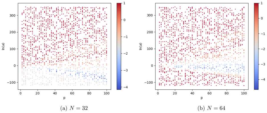
Through linear stability analysis we prove that the instabilities are unavoidable for any space-time sufficiently close to FLRW while we find that this approach can be stable for Gowdy space-times depending on the initial time choice. Additionally, we present numerical evidence that certain subclasses of the algebraic-hyperbolic formulation, when combined with a Fourier-based method of lines, are numerically stable.
What carries the argument
The algebraic-hyperbolic formulation of the Einstein constraint equations, discretized by a pseudo-spectral method of lines and subjected to linear stability analysis.
If this is right
- The standard algebraic-hyperbolic formulation cannot be used reliably for initial data construction near FLRW with Fourier-based discretizations.
- Stability for Gowdy spacetimes requires a suitable choice of initial time slice.
- Certain subclasses of the formulation remain candidates for stable numerical initial data sets in inhomogeneous cosmologies.
Where Pith is reading between the lines
- Alternative spatial discretizations such as finite differences might evade the reported instabilities even if the continuous system is marginally stable.
- The dependence on background geometry suggests that hyperbolic constraint formulations must be re-examined for each class of cosmological symmetry.
- The stable subclasses identified numerically could be tested on spacetimes with different topologies or matter sources to check broader applicability.
Load-bearing premise
The spacetime is close enough to FLRW that linear perturbations around it capture the dominant numerical behavior.
What would settle it
A long-term stable numerical evolution of the full algebraic-hyperbolic system for a spacetime arbitrarily close to FLRW, using the same Fourier method of lines, would falsify the unavoidability claim.
Figures








read the original abstract
In this work, we study of the algebraic-hyperbolic formulation of the Einstein constraint equations for numerically constructing initial data sets for inhomogeneous cosmological space-times with $\mathbb{T}^3$ topology. We implement a pseudo-spectral method of lines based on the discrete Fourier transform and find that the scheme exhibits pathological instabilities. Through linear stability analysis, we prove that the instabilities are unavoidable for any space-time sufficiently close to FLRW while we find that this approach can be stable for Gowdy space-times depending on the initial time choice. Additionally, we present numerical evidence that certain subclasses of the algebraic-hyperbolic formulation, when combined with a Fourier-based method of lines, are numerically stable, thus offering a potential new path for computing initial data sets for inhomogeneous cosmological space-times.
Editorial analysis
A structured set of objections, weighed in public.
Referee Report
Summary. The manuscript studies the algebraic-hyperbolic formulation of the Einstein constraint equations on T^3 topologies for cosmological initial data. A pseudo-spectral method of lines based on the discrete Fourier transform is implemented and shown to exhibit pathological instabilities. Linear stability analysis is invoked to prove that instabilities are unavoidable for any spacetime sufficiently close to FLRW, while stability is possible for Gowdy spacetimes depending on the initial time slice. Numerical evidence is presented that certain subclasses of the formulation remain stable under the same discretization.
Significance. If the linear analysis rigorously establishes persistence of instabilities under small deviations from FLRW, the result would be significant for numerical relativity: it would identify a structural limitation of the algebraic-hyperbolic system near the most common cosmological backgrounds and point to stable subclasses as a practical alternative. The combination of analytic proof and targeted numerical tests is a positive feature when the mode-coupling question is resolved.
major comments (2)
- [linear stability analysis (abstract and implementation paragraph)] Abstract and linear stability analysis section: the central claim that instabilities are 'unavoidable for any space-time sufficiently close to FLRW' is load-bearing. The analysis appears to be performed on the exact homogeneous FLRW background (where DFT modes remain eigenmodes). Small spatial inhomogeneities introduce off-diagonal coupling in the mode equations; without a first-order perturbation of the background coefficients to verify that unstable eigenvalues persist, the extension to nearby inhomogeneous spacetimes is not established.
- [numerical results section] Numerical evidence paragraph: the reported stability for certain subclasses is presented as offering a 'potential new path,' yet no quantitative error norms, convergence rates, or comparison against a known exact solution (e.g., perturbed FLRW) are referenced. This weakens the practical utility claim.
minor comments (2)
- [abstract] The abstract states 'we prove' but does not indicate whether the linear analysis includes a systematic expansion in spatial inhomogeneity amplitude; this should be clarified in the main text.
- [formulation section] Notation for the algebraic-hyperbolic system variables should be introduced once with explicit reference to the original formulation paper.
Simulated Author's Rebuttal
We thank the referee for their thorough review and valuable comments on our manuscript. We address each major comment below and indicate the revisions we plan to make.
read point-by-point responses
-
Referee: Abstract and linear stability analysis section: the central claim that instabilities are 'unavoidable for any space-time sufficiently close to FLRW' is load-bearing. The analysis appears to be performed on the exact homogeneous FLRW background (where DFT modes remain eigenmodes). Small spatial inhomogeneities introduce off-diagonal coupling in the mode equations; without a first-order perturbation of the background coefficients to verify that unstable eigenvalues persist, the extension to nearby inhomogeneous spacetimes is not established.
Authors: We agree with the referee that our linear stability analysis is conducted on the homogeneous FLRW background, where the discrete Fourier modes are exact eigenmodes. The extension to spacetimes sufficiently close to FLRW relies on the expectation that the unstable eigenvalues will persist under small perturbations of the coefficients. However, as noted, a first-order perturbative analysis of the coupled mode equations would provide a more rigorous justification. We will revise the manuscript to explicitly acknowledge this limitation of the current analysis and to discuss the conditions under which the instabilities are expected to persist, including a sketch of how a perturbative treatment could be carried out. revision: yes
-
Referee: Numerical evidence paragraph: the reported stability for certain subclasses is presented as offering a 'potential new path,' yet no quantitative error norms, convergence rates, or comparison against a known exact solution (e.g., perturbed FLRW) are referenced. This weakens the practical utility claim.
Authors: We acknowledge that the numerical evidence for the stability of certain subclasses could be strengthened with quantitative measures. In the revised version, we will include L^2 error norms, demonstrate convergence rates with respect to the number of Fourier modes, and provide comparisons to exact solutions for the Gowdy spacetimes and other stable cases where possible. This will better support the claim of numerical stability and the potential utility of these subclasses. revision: yes
Circularity Check
No circularity: linear analysis is independent of numerics
full rationale
The paper derives its main result (instabilities unavoidable near FLRW) via linear stability analysis of the algebraic-hyperbolic system and separately reports numerical evidence for stability in Gowdy cases. No quoted step shows a parameter fitted to data then renamed as prediction, a self-definitional loop, or a load-bearing self-citation chain that reduces the claim to its own inputs. The derivation remains self-contained as a direct mathematical analysis of the PDE system.
Axiom & Free-Parameter Ledger
axioms (2)
- domain assumption The Einstein constraint equations admit an algebraic-hyperbolic formulation suitable for numerical evolution.
- domain assumption Linear stability analysis of the semi-discrete system correctly captures the behavior of the full nonlinear numerical scheme near FLRW.
Reference graph
Works this paper leans on
-
[1]
M. Alcubierre. Introduction to 3+ 1 numerical relativity , volume 140. OUP Oxford, 2008
work page 2008
-
[2]
M. Alcubierre, G. Allen, C. Bona, D. Fiske, T. Goodale, F. S. Guzm´ an, I. Hawke, S. H. Hawley, S. Husa, M. Koppitz, C. Lechner, D. Pollney, D. Rideout, M. Salgado, E. Schnetter, E. Seidel, H. aki Shinkai, D. Shoemaker, B. Szil´ agyi, R. Takahashi, and J. Winicour. Towards 31 standard testbeds for numerical relativity. Classical and Quantum Gravity , 21(2...
work page 2003
-
[3]
T. W. Baumgarte and S. L. Shapiro. Numerical relativity: solving Einstein’s equations on the computer. Cambridge University Press, 2010
work page 2010
- [4]
- [5]
- [6]
- [7]
-
[8]
K. Csuk´ as and I. R´ acz. Numerical investigations of the asymptotics of solutions to the evolutionary form of the constraints. Classical and Quantum Gravity , 37(15):155006, 2020
work page 2020
-
[9]
K. Csuk´ as and I. R´ acz. Is it possible to construct asymptotically flat initial data using the evolutionary forms of the constraints? Physical Review D, 107(8):084013, 2023
work page 2023
-
[10]
M. P. Do Carmo and J. Flaherty Francis. Riemannian geometry, volume 6. Springer, 1992
work page 1992
- [11]
-
[12]
R. Durrer. The Cosmic Microwave Background . Cambridge University Press, 2008
work page 2008
-
[13]
D. Garfinkle and L. Mead. Cosmological initial data for numerical relativity. Phys. Rev. D , 102:044022, Aug 2020
work page 2020
-
[14]
D. J. Higham and L. N. Trefethen. Stiffness of odes. BIT Numerical Mathematics , 33:285– 303, 1993
work page 1993
-
[15]
D. A. Kopriva. Implementing spectral methods for partial differential equations: Algorithms for scientists and engineers . Springer Science & Business Media, 2009
work page 2009
- [16]
-
[17]
H. J. Macpherson, P. D. Lasky, and D. J. Price. Inhomogeneous cosmology with numerical relativity. Phys. Rev. D , 95:064028, Mar 2017
work page 2017
-
[18]
H. J. Macpherson, D. J. Price, and P. D. Lasky. Einstein’s universe: Cosmological structure formation in numerical relativity. Phys. Rev. D , 99:063522, Mar 2019
work page 2019
-
[19]
F. K. Morton and B. MJ. Lax-stability vs. eigenvalue stability of spectral methods. 32
-
[20]
P. J. E. Peebles. The large-scale structure of the universe , volume 98. Princeton university press, 2020
work page 2020
-
[21]
I. R´ acz. Cauchy problem as a two-surface based ‘geometrodynamics’.Classical and Quantum Gravity, 32(1):015006, 2014
work page 2014
-
[22]
I. R´ acz. Is the bianchi identity always hyperbolic? Classical and Quantum Gravity , 31(15):155004, 2014
work page 2014
-
[23]
I. R´ acz. Constraints as evolutionary systems.Classical and Quantum Gravity, 33(1):015014, 2015
work page 2015
-
[24]
S. C. Reddy and L. N. Trefethen. Stability of the method of lines. Numerische Mathematik, 62(1):235–267, 1992
work page 1992
-
[25]
H. Ringstr¨ om. Cosmic censorship for gowdy spacetimes. Living Reviews in Relativity , 13:1– 59, 2010
work page 2010
- [26]
-
[27]
M. Taylor. Partial differential equations II: Qualitative studies of linear equations , volume
-
[28]
Springer Science & Business Media, 2013
work page 2013
-
[29]
L. N. Trefethen. Spectral methods in MATLAB . SIAM, https://doi.org/10.1137/1.9780898719598, 2000
-
[30]
L. N. Trefethen and M. Embree. Spectra and Pseudospectra: The Behavior of Nonnormal Matrices and Operators. Princeton University Press, 2005
work page 2005
-
[31]
R. M. Wald. General Relativity. Chicago Univ. Pr., Chicago, USA, 1984. 33 A Aliasing error and filtering strategy Aliasing error emerges from the non-linearities of the PDE and is due to the finiteness of the grid (see [7, 15]). Since our equations (eqs. (6) to (8)) are non-linear, determine the relevance of this error is important to obtain accurate nume...
work page 1984
discussion (0)
Sign in with ORCID, Apple, or X to comment. Anyone can read and Pith papers without signing in.