pith. sign in

arxiv: 2408.01914 · v4 · submitted 2024-07-13 · 🧮 math.NA · cs.AI· cs.NA

Partial-differential-algebraic equations of nonlinear dynamics by Physics-Informed Neural-Network: (I) Operator splitting and framework assessment

Pith reviewed 2026-05-23 22:55 UTC · model grok-4.3

classification 🧮 math.NA cs.AIcs.NA
keywords physics-informed neural networksoperator splittingpartial differential algebraic equationsKirchhoff rodDeepXDEJAXnonlinear dynamicsPDAE
0
0 comments X

The pith

Derivative operator splitting lets PINNs solve PDAEs directly from the highest-level balance-of-momenta form

A machine-rendered reading of the paper's core claim, the machinery that carries it, and where it could break.

The paper introduces PINN constructions that split derivative operators to handle partial-differential-algebraic equations, using the nonlinear Kirchhoff rod as the test case. These constructions start from the balance-of-momenta equations rather than requiring successive substitutions to reach a lowest-level form. The methods are shown to avoid the pathological failures observed when DeepXDE with TensorFlow is applied to the same problems. A JAX implementation is supplied together with a normalized training protocol that the authors codified from their runs. If the approach holds, the usual workflow of hand derivation followed by weak-form discretization can be skipped for this class of nonlinear dynamics problems.

Core claim

Several new PINN formulations are obtained by splitting the derivative operators in the PDAE system; these formulations evolve from low-level to high-level versions and allow the balance-of-momenta equations themselves to be used as the starting point. The resulting networks are applied to the nonlinear Kirchhoff rod, the JAX script reproduces results without the instabilities seen in DeepXDE-TensorFlow, and the higher-level forms turn out to be more efficient than the lower-level ones in that implementation.

What carries the argument

Derivative operator splitting applied to construct the residual terms of a PINN loss directly from high-level PDAE balance equations

If this is right

  • The balance-of-momenta form can be fed directly to the network, eliminating the error-prone manual reduction to lower-level equations.
  • Higher-level forms become practically usable and sometimes more efficient than their reduced counterparts.
  • A standardized normalization step in the training loop makes learning-rate choices reproducible across runs.
  • The JAX script avoids the specific convergence failures documented for DeepXDE with TensorFlow on the same rod problem.

Where Pith is reading between the lines

These are editorial extensions of the paper, not claims the author makes directly.

  • The same splitting pattern could be tested on other PDAE systems such as beams with large deformation or fluid-structure interaction.
  • Codifying the training normalization may shorten the trial-and-error phase when PINNs are first applied to a new nonlinear model.
  • If the higher-level forms remain stable, automatic code generation from symbolic balance laws could become feasible without intermediate reduction steps.

Load-bearing premise

The split-operator PDAE forms together with the JAX training procedure can produce accurate solutions for the Kirchhoff rod system without new instabilities or extensive per-problem retuning.

What would settle it

Execute the supplied JAX script on the Kirchhoff rod PDAE and compare the resulting time histories of displacement and rotation against an independent reference solution obtained by a conventional finite-element discretization; systematic deviation beyond discretization error falsifies the claim.

Figures

Figures reproduced from arXiv: 2408.01914 by Alexander Humer, Loc Vu-Quoc.

Figure 1
Figure 1. Figure 1: Geometrically-exact beam without shear deformation. Section 2.1. Shear forces introduced for equilibrium. Section 2.2: Inconsistency in Kirchhoff rod (large deformation) and Euler-Bernoulli (small deformation) beam theories [PITH_FULL_IMAGE:figures/full_fig_p005_1.png] view at source ↗
Figure 2
Figure 2. Figure 2: Geometrically-exact beam with shear deformation. The deformed configuration (solid line) is superposed on the initial configuration (dotted line) of unit length (which could be multiplied by dX). Shear deformation is the difference between the angle α of the deformed centroidal line and the rotation θ of the cross section. Spatial strains {γ1, γ2} and material strains {Γ1, Γ2}, such that γ = γ1e1 + γ2e2 = … view at source ↗
Figure 3
Figure 3. Figure 3: DDE-T. Pinned-pinned elastic bar, axial motion. Model summary. Feedforward neural network (fnn). Remark 5.4. Section 5.3.1, Form 1. Dense-connection layers, each between two consecutive layers of neurons. Network: Remark 5.3, n_inp=2, W=64, H=4, n_out=1, 12737 parameters. Six neuron layers (1 input, 4 hidden, 1 output), five connection layers (pairs of consecutive neuron layers). (23721R1-1) Remark 5.5. Da… view at source ↗
Figure 4
Figure 4. Figure 4: Optimization learning-rate scheduling. Section 5.2. Cycles and periods. After an initial-learning rate for a number of cycles was chosen, e.g., init_lr = 0.001, in any given period (p) within a cycle, the learning rate ϵ(p-1) at the end of the previous period (p-1) is decayed to the value ϵ(p) = fdecay · ϵ(p-1), with fdecay being a decay factor less than one, following a decay function, such as the “invers… view at source ↗
Figure 5
Figure 5. Figure 5: Axial motion of elastic bar. Section 5.3. Mathematica solutions. Eq. (64) with slenderness s = 1 and distributed load f X = 1/2. Two vibration periods for each set of boundary conditions. Left: Pinned-pinned bar, with X ∈ [0, 1] and t ∈ [0, 4]. Right: Pinned￾free bar, with X ∈ [0, 1] and t ∈ [0, 8] [PITH_FULL_IMAGE:figures/full_fig_p019_5.png] view at source ↗
Figure 6
Figure 6. Figure 6: DDE-T. Pinned-pinned bar, cyclic annealing (CA). Static-shape (left), static midspan displacement (right), Step 50,000. ⋆ Section 5.3.2, Form 2a. Remarks 3.3 (Static solution), 5.20 (How to avoid). Network: ⋆ Remarks 5.3, 5.5, T=4, W=32, H=2, n_out=2, He-uniform initializer, 1,218 parameters, regular grid. Training: ⋆ Remark 5.6, LRS 1, init_lr=0.07, n-cycles=2, N_steps=50,000. • [PITH_FULL_IMAGE:figures/… view at source ↗
Figure 7
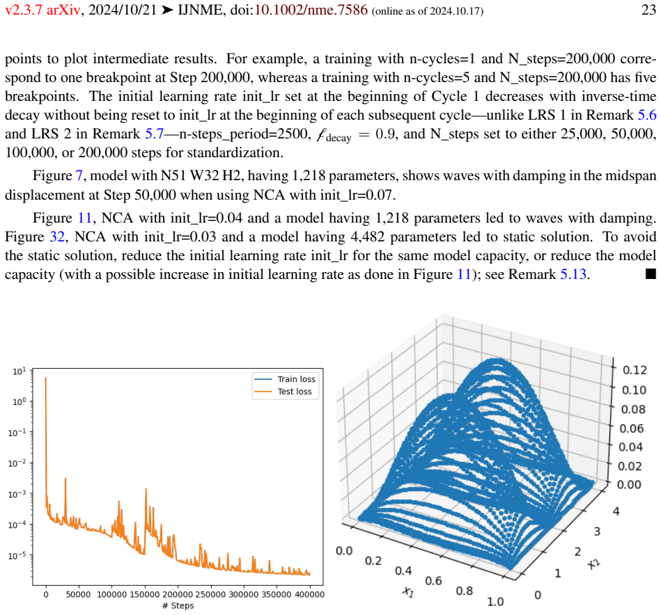
Figure 7. Figure 7: DDE-T. Pinned-pinned bar, No cyclic annealing (NCA). Shape (left), midspan dis￾placement (right), Step 50,000, waves with damping. ⋆ Section 5.3.2, Form 2a. Remark 5.14, Damping. Network: ⋆ Remarks 5.3, 5.5, T=4, W=32, H=2, n_out=2, He-uniform initial￾izer, 1,218 parameters, regular grid. Training: Remark 5.8, LRS 3, init_lr=0.07, n-cycles=2, N_steps=50,000. • [PITH_FULL_IMAGE:figures/full_fig_p020_7.png] view at source ↗
Figure 8
Figure 8. Figure 8: DDE-T. Pinned-pinned bar, cyclic annealing (CA). Loss function (left), midspan displacement, Step 200,000 (right), waves with damping. ⋆ Section 5.3.2, Form 2a. Network: ⋆ Remarks 5.3, 5.5, T=4, W=64, H=2, n_out=2, He-uniform initializer, 4,482 parameters, ⋆ regular grid. Training: ⋆ Remark 5.6, LRS 1 (CA), init_lr=0.03. • [PITH_FULL_IMAGE:figures/full_fig_p020_8.png] view at source ↗
Figure 9
Figure 9. Figure 9: DDE-T. Pinned-pinned bar, cyclic annealing (CA). Loss function (left), midspan displacement, Step 200,000 (right), static solution. ⋆ Section 5.3.2, Form 2a. Network: ⋆ Remarks 5.3, 5.5, T=4, W=32, H=2, n_out=2, He-uniform initializer, 1,218 parameters, ⋆ regular grid. Training: ⋆ Remark 5.6, LRS 1 (CA), init_lr=0.04. • [PITH_FULL_IMAGE:figures/full_fig_p021_9.png] view at source ↗
Figure 10
Figure 10. Figure 10: DDE-T. Pinned-pinned bar, Varying init_lr cyclic annealing (VCA). Loss func￾tion (left), midspan displacement (right), Step 200,000, waves, small damping. Section 5.3.2, Form 2a. ⋆ Remark 5.14, Damping. Network: Remarks 5.3, 5.5, T=4, W=32, H=2, n_out=2, He-uniform initializer, 1,218 parameters, regular grid. Training: ⋆ Remark 5.7, LRS 2 (VCA), init_lr=[0.04, 0.03, 0.02, 0.01, 0.005]. • [PITH_FULL_IMAGE… view at source ↗
Figure 11
Figure 11. Figure 11: DDE-T. Pinned-pinned bar, NO cyclic annealing (NCA). Loss function (left), midspan displacement, Step 200,000 (right), waves with damping. ⋆ Section 5.3.2, Form 2a. Network: ⋆ Remarks 5.3, 5.5, T=4, W=32, H=2, n_out=2, He-uniform initializer, 1,218 pa￾rameters, ⋆ regular grid. Training: ⋆ Remark 5.8, LRS 3 (NCA), init_lr=0.04. • [PITH_FULL_IMAGE:figures/full_fig_p022_11.png] view at source ↗
Figure 12
Figure 12. Figure 12: DDE-T. Pinned-pinned bar, Extended learning-rate schedule (ELRS). Loss func￾tion (left), shape, Step 400,000 (right). ⋆ Section 5.3.2, Form 2a. Network: ⋆ Remarks 5.3, 5.5, T=4, W=32, H=2, n_out=2, He-uniform initializer, 1,218 parameters, ⋆ regular grid. Train￾ing: ⋆ Remarks 5.6 (LRS 1), 5.9 (ELRS), init_lr=0.02, Cycles 1-5 (CA), Cycles 6-9 (NCA), N_steps=400,000. ⋆ Lowest total loss 2.19e-06, Step 400,0… view at source ↗
Figure 13
Figure 13. Figure 13: DDE-T. Pinned-pinned bar, ELRS. Midspan displacements: Step 200,000 (left), Step 300,000 (right). Section 5.3.2, Form 2a. Network: ⋆ Remarks 5.3, 5.5, T=4, W=32, H=2, n_out=2, He-uniform initializer, 1,218 parameters, ⋆ regular grid. Training: ⋆ Re￾marks 5.6 (LRS 1), 5.9 (ELRS), init_lr=0.02, n-cycles=9, Cycles 1-5 (CA), Cycles 6-9 (NCA), N_steps=400,000. • [PITH_FULL_IMAGE:figures/full_fig_p024_13.png] view at source ↗
Figure 14
Figure 14. Figure 14: DDE-T. Pinned-pinned bar, ELRS. Velocity (left) and very-good midspan dis￾placement (right), Step 400,000. ⋆ Section 5.3.2, Form 2a. Network: ⋆ Remarks 5.3, 5.5, T=4, W=32, H=2, n_out=2, He-uniform initializer, 1,218 parameters, regular grid. Training: ⋆ Re￾marks 5.6, (LRS 1), 5.9 (ELRS), init_lr=0.02, n-cycles=9, Cycles 1-5 (CA), Cycles 6-9 (NCA), N_steps=400,000. • [PITH_FULL_IMAGE:figures/full_fig_p02… view at source ↗
Figure 15
Figure 15. Figure 15: DDE-T. Pinned-pinned bar, lower-capacity network 1. Shape (left), midspan dis￾placement (right), Step 200,000. ⋆ Remark 5.13, Optimal capacity. Remark 5.16, Unstable solution. Section 5.3.2, Form 2a. Network: ⋆ Remarks 5.3, 5.5, T=4, W=64, H=2, n_out=2, He-uniform initializer, 4,482 parameters, ⋆ regular grid. Training: Remark 5.6 (LRS 1), init_lr=0.01. ⋆ Lowest loss value 2.12e-06, Step 200,000. Total GP… view at source ↗
Figure 16
Figure 16. Figure 16: DDE-T. Pinned-pinned bar, lower-capacity network 2. Midspan displacement, damping, Step 200,000. ⋆ Remark 5.13, Optimal capacity. Section 5.3.2, Form 2a. Network: Remark 5.3, 5.5, T=4, W=32, H=2, n_out=2, He-uniform initializer, 1,218 parameters, regular grid. Training: init_lr=0.01. Left: Remark 5.6, LRS 1 (CA) (23816R2a-1); Right: Remark 5.8, LRS 3 (NCA) (23816R2b-1). • Quasi-perfect solutions [PITH_FU… view at source ↗
Figure 17
Figure 17. Figure 17: DDE-T. Pinned-pinned bar, damping in low-capacity networks. Shape (left), midspan displacement (right, damping), Step 200,000. ⋆ Remark 5.14, Damping. Sec￾tion 5.3.2, Form 2a. Network: Remarks 5.3, 5.5, T=4, W=32, H=2, n_out=2, He-uniform initializer, 1,218 parameters, random grid. Training: Remark 5.6, LRS 1, init_lr=0.03. • [PITH_FULL_IMAGE:figures/full_fig_p027_17.png] view at source ↗
Figure 18
Figure 18. Figure 18: DDE-T. Pinned-pinned bar, damping in low-capacity networks. Loss function (left), velocity (right), Step 200,000. Remark 5.14, Damping. ⋆ Section 5.3.2, Form 2a. Net￾work: Remarks 5.3, 5.5, T=4, W=32, H=2, n_out=2, He-uniform initializer, 1,218 parameters, random grid. Training: ⋆ Remark 5.6, LRS 1, init_lr=0.03. • [PITH_FULL_IMAGE:figures/full_fig_p028_18.png] view at source ↗
Figure 19
Figure 19. Figure 19: DDE-T. Pinned-pinned bar, damping in low-capacity networks. Left: Waves, damping, Step 200,000. Right: Static solution, Step 50,000. ⋆ Remark 5.14, Damping. Sec￾tion 5.3.2, Form 2a. Network: Remarks 5.3, 5.5, T=4, W=32, H=2, n_out=2, He-uniform initializer, 1,218 parameters, random grid (left), regular grid (right). Training: ⋆ Left: Re￾mark 5.6, LRS 1, init_lr=0.001 (23817R2-1). Right: Remark 5.8, LRS 3,… view at source ↗
Figure 20
Figure 20. Figure 20: DDE-T. Pinned-pinned bar. Shape (left), midspan displacement shifted to the right with small amplification (right), Step 100,000. ⋆ Section 5.3.1, Form 1. Network: Re￾marks 5.3, 5.5, T=4, W=64, H=4, n_out=1, Glorot-uniform initializer, 12,737 parameters, regu￾lar grids. Training: ⋆ Remark 5.8, LRS 3 (NCA), init_lr=0.001, n-cycles=3, N_steps=100,000. ⋆ PDE loss 2.20e-06, Cycle 3 GPU time 154 sec. ▷ [PITH_… view at source ↗
Figure 21
Figure 21. Figure 21: DDE-T. Pinned-pinned bar. Shape (left), midspan displacement shifted to the right with small amplification (right), Step 200,000. ⋆ Section 5.3.1, Form 1. Network: Re￾marks 5.3, 5.5, T=4, H=4, W=64, n_out=1, Glorot-uniform initializer, 12,737 parameters fixed random grid. Training: ⋆ Remark 5.6, LRS 1 (CA), init_lr=0.001. ⋆ Lowest total loss 4.31e-06, Step 200,000 (sum of 5 losses). ⋆ Total GPU time 621 s… view at source ↗
Figure 22
Figure 22. Figure 22: DDE-T. Pinned-pinned bar, continued shift & amplification. ⋆ Midspan displace￾ments: Step 50,000 (left), Step 400,000 (right). ⋆ Section 5.3.1, Form 1: Hidden parameters (s, c, a), time shift s, vertical shift c, amplification a, quasi-perfect peak-to-peak amplitude A. Network: Remarks 5.3, 5.5, T=4 W=64, H=4, n_out=1, He-uniform initializer, 12,737 pa￾rameters, regular grid. Training: Remark 5.6, LRS 3 (… view at source ↗
Figure 23
Figure 23. Figure 23: DDE-T. Pinned-pinned bar. Form 1. Appendix 1, Analysis. Scaled shift￾amplification parameters (s, c, a) and initial velocity increase with training step number (left), while the Total loss continues to decrease (right). All parameters p, such as time shift s, vertical shift c, amplification factor a and thus peak-to-peak amplitude aA, and initial velocity, were scaled to fit in the chart. • [PITH_FULL_IM… view at source ↗
Figure 24
Figure 24. Figure 24: JAX. Pinned-pinned bar, No shift & amplification, Remark 5.17. ⋆ Left: Loss function. Right: Step 198,000, lowest loss 1.724e-06, midspan displacement, times at local maxima (1., 3.), times at local minima (0., 2., 4.), damping%=1.7%, Quality: Good. ⋆ Sec￾tion 5.3.1, Form 1. Network: Remarks 5.3, 5.5, T=4, W=64, H=4, Uniform initializer, 12,737 parameters, random grid. Training: Remark 5.10, LRS 4, init_l… view at source ↗
Figure 25
Figure 25. Figure 25: DDE-T. Pinned-pinned bar, early stopping. ⋆ Left: Loss function, lowest value 2.30e-05 at Step 24,000, value 0.25 at Step 100,000, divergence. Right: Shape, Step 24,000. ⋆ Section 5.3.1, Form 1. Network: Remarks 5.3, 5.5, T=4, W=64, H=4, n_out=1, He-uniform initializer, 12,737 parameters, regular grid. Training: Remark 5.6, LRS 1 (CA), init_lr=0.03. • [PITH_FULL_IMAGE:figures/full_fig_p034_25.png] view at source ↗
Figure 26
Figure 26. Figure 26: DDE-T. Pinned-pinned bar. Midspan displacement, damping, Step 25,000 (left), zero midspan displacement, Step 100,000 (divergence, right). Section 5.3.1, Form 1. Network: Remarks 5.3, 5.5, T=4, W=64, H=4, n_out=1, He-uniform initializer, 12,737 parameters, regu￾lar grid. Training: Remark 5.6, LRS 1 (CA), init_lr=0.03. • [PITH_FULL_IMAGE:figures/full_fig_p034_26.png] view at source ↗
Figure 27
Figure 27. Figure 27: DDE-T, Form 1, pinned-free bar, static solutions (Remark 5.19, Section 5.3.1). • SubFigs. 27a-27b: Shape, free-end displacement, Step 25000; GPU time 655 sec (Deter￾ministic mode) for 200,000 steps. (2398R2a). Shape, free-end disp, step number for other pairs: (27c-27d) (2398R2b), (27e-27f) (2398R2c), (27g-27h) (2398R2d). • Network: Remarks 5.3, 5.5, T=8, W=64, H=2, n_out=1, Glorot-uniform initializer, ra… view at source ↗
Figure 28
Figure 28. Figure 28: JAX. Form 1, pinned-free bar. Remark 5.10 (LRS 4). • SubFigs 28a-28b: 12,737 params, Step 49,000, Cycle 2 lowest loss 5.324e-06, damping%=0.25%, Quasi-perfect, GPU time 161 sec. Network: Remarks 5.3, 5.5, T=8, W=64, H=2, n_out=1, Uniform initializer, random grid. Training: Remark 5.10 LRS 4, init_lr=0.002, factor_lr=[0.9, 0.9, 0.9, 0.8, 0.8, 1, 1, 1, 1]. (23916R1a.4). ⋆ SubFigs 28c-28d: Cycle 3 lowest los… view at source ↗
Figure 29
Figure 29. Figure 29: DDE-T. Pinned-pinned bar, static solution. Loss function (left), static solution (right), Step 50,000, end of Cycle 2. ⋆ Remark 3.3, Static solution; Remark 5.20, How to avoid. Section 5.3.2, Form 2a. Network: Remarks 5.3, 5.5, T=4, W=64, H=4, n_out=2, He-uniform initializer, 12,802 parameters, ⋆ regular grid. Training: Remark 5.8, LRS 3, init_lr=0.01, n￾cycles=2, N_steps=50,000. • [PITH_FULL_IMAGE:figur… view at source ↗
Figure 30
Figure 30. Figure 30: DDE-T. Pinned-pinned bar, static solution. Essentially-zero velocity (left); static midspan displacement (right), Step 50,000, end of Cycle 2. ⋆ Remark 3.3, Static solution; Remark 5.20, How to avoid. Section 5.3.2, Form 2a. Network: Remarks 5.3, 5.5, T=4, W=64, H=4, n_out=2, He-uniform initializer, 12,802 parameters, ⋆ regular grid. Training: Remark 5.8, LRS 3, init_lr=0.01, n-cycles=2, N_steps=50,000. •… view at source ↗
Figure 31
Figure 31. Figure 31: DDE-T. Pinned-pinned bar. Pre-static midspan-displacement time histories at Step 25,000 (end of Cycle 1). ⋆ Remarks 3.3, 5.20. Section 5.3.2, Form 2a. ⋆ Network: Remark 5.3, 5.5, T=4, W=64, H=2, n_out=2, He-uniform initializer, 4,482 parameters, regu￾lar grid. Training: Remark 5.8, LRS 3, init_lr=0.03. ⋆ Left: n-cycles=5, N_steps=200,000; Figures 32-33, Step 200,000. (23815R3a-1). ⋆ Right: n-cycles=1, N_s… view at source ↗
Figure 32
Figure 32. Figure 32: DDE-T. Pinned-pinned bar, no cyclic annealing (NCA). Loss function (left) and static-shape (right), Step 200,000. ⋆ Remarks 3.3, 5.20. Section 5.3.2, Form 2a. Network: Remarks 5.3, 5.5, T=4, W=64, H=2, n_out=2, He-uniform initializer, 4,482 parameters, regular grid. ⋆ Training: Remark 5.8, LRS 3, init_lr=0.03. • [PITH_FULL_IMAGE:figures/full_fig_p039_32.png] view at source ↗
Figure 33
Figure 33. Figure 33: DDE-T. Pinned-pinned bar, no cyclic annealing (NCA). ⋆ Essentially-zero Veloc￾ity (left), static midspan displacement (right), Step 200,000. ⋆ Remarks 3.3, 5.20. Section 5.3.2, Form 2a. Network: Remarks 5.3, 5.5, T=4, W=64, H=2, n_out=2, He-uniform initializer, 4,482 parameters, regular grid. Training: Remark 5.8, LRS 3, init_lr=0.03. • [PITH_FULL_IMAGE:figures/full_fig_p040_33.png] view at source ↗
Figure 34
Figure 34. Figure 34: DDE-T. Pinned-pinned bar. Shape (left), midspan displacement (right), small damping, Step 250,000. ⋆ Section 5.3.2, Form 2a. Network: Remarks 5.3, 5.5, T=4, W=64, H=4, n_out=2, He-uniform initializer, 12,802 parameters, regular grid. Training: ⋆ Remarks 5.6 (LRS 1), 5.9 (ELRS), init_lr=0.001, Cycles 1-5 (CA), Cycle 6 (NCA), N_steps=250,000. ⋆ Lowest total loss 2.55e-06, Step 250,000 (sum of 6 losses). • F… view at source ↗
Figure 35
Figure 35. Figure 35: DDE-T. Pinned-pinned bar. Step 200,000: Shape (left), midspan displace￾ment (right), visually quasi-perfect. ⋆ Remark 5.13, Optimal capacity. Remark 5.16, Un￾stable solution. Remark 5.20, Avoiding static solution. Section 5.3.2, Form 2a. Net￾work: ⋆ Remarks 5.3, 5.5, T=4, W=64, H=4, n_out=2, He-uniform initializer, 12,802 pa￾rameters, ⋆ random grid. Training: ⋆ Remark 5.8 LRS 3 (NCA), init_lr=0.01. n-cycl… view at source ↗
Figure 36
Figure 36. Figure 36: DDE-T. Pinned-pinned bar. Left: Loss function. Right: Step 146,000, midspan displacement (right), damping%=0.3%, Quasi-perfect. ⋆ Section 5.3.2, Form 2a. Network: ⋆ Remarks 5.3, 5.5, T=4, W=64, H=4, n_out=2, He-uniform initializer, 12,802 parameters, ⋆ random grid. Training: ⋆ Remark 5.8 LRS 3 (NCA), init_lr=0.01. ⋆ Total loss 0.722e-06, Step 146,000 (sum of 6 losses). Total GPU time 442 sec. • [PITH_FUL… view at source ↗
Figure 37
Figure 37. Figure 37: DDE-T. Pinned-free bar. He-uniform initializer. ⋆ Static shape (left), free-end displacement (right), Step 25,000, end of Cycle 1. Section 5.3.2, Form 2a. Network: Re￾marks 5.3, 5.5, T=8, W=64, H=4, n_out=2, He-uniform initializer, 12,802 parameters, regular grid. Training: Remark 5.8, LRS 3, init_lr=0.005. • [PITH_FULL_IMAGE:figures/full_fig_p042_37.png] view at source ↗
Figure 38
Figure 38. Figure 38: DDE-T. Pinned-free bar. He-uniform initializer. ⋆ Step 100,000: Shape (left), free-end displacement (right), damping%=0.14%, Quasi-perfect. Section 5.3.2, Form 2a. Net￾work: Remarks 5.3, 5.5, T=8, W=64, H=4, n_out=2, He-uniform initializer, 12,802 parameters, random grid. Training: Remark 5.8, LRS 3, init_lr=0.005, Cycle 3 lowest loss 2.472e-06, GPU time 318 sec. (2395R3b-1) • (Cycle 5 lowest loss 1.268e-… view at source ↗
Figure 39
Figure 39. Figure 39: DDE-T. Pinned-pinned bar. Step 88,000: “t.h.” = time history. SubFig. 39e, midspan displacement t.h., damping%=0.1%, Quasi-perfect. ⋆ Section 5.3.2, Form 3. Network: ⋆ Remarks 5.3, 5.5, T=4, W=64, H=4, n_out=3, He-uniform initializer, 12,867 parameters, ⋆ random grid. Training: ⋆ Remark 5.8 LRS 3 (NCA), init_lr=0.01. ⋆ Total loss 1.179e-06, (sum of 7 losses). Total GPU time 278 sec. • The above is a good … view at source ↗
Figure 40
Figure 40. Figure 40: DDE-T. Pinned-pinned bar, VCA. Shape (left), midspan displacement, Step 200,000 (right), waves, small damping. ⋆ Section 5.3.4, Form 3. Remark 5.14, Damping. Network: Remarks 5.3, 5.5, T=4, W=32, H=2, n_out=2, He-uniform initializer, 1,251 param￾eters, ⋆ regular grid. Training: ⋆ Remark 5.7, LRS 2 (VCA), init_lr=[0.04, 0.03, 0.02, 0.01, 0.005]. ⋆ Lowest total loss 4.31e-06, Step 200,000 (sum of 7 losses).… view at source ↗
Figure 41
Figure 41. Figure 41: DDE-T. Pinned-pinned bar, VCA. Velocity (left), slope (right), Step 200,000, waves, small damping. ⋆ Section 5.3.4, Form 3. Network: ⋆ Remarks 5.3, 5.5, T=4, W=32, H=2, n_out=2, He-uniform initializer, 1,251 parameters, ⋆ regular grid. Training: ⋆ Re￾mark 5.7, LRS 2 (VCA), init_lr=[0.04, 0.03, 0.02, 0.01, 0.005]. • [PITH_FULL_IMAGE:figures/full_fig_p044_41.png] view at source ↗
Figure 42
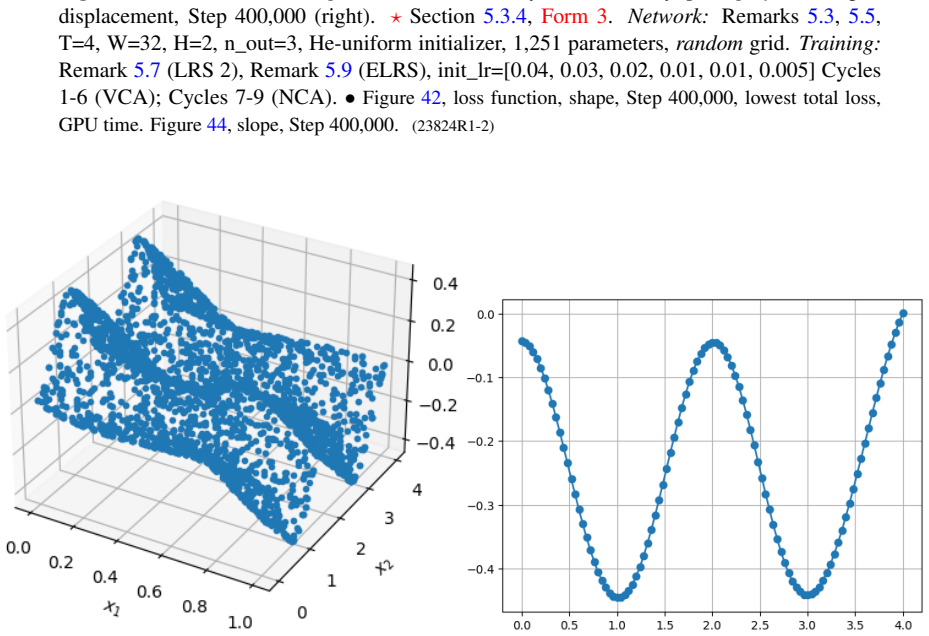
Figure 42. Figure 42: DDE-T. Pinned-pinned bar. Loss function (left), shape, Step 400,000 (right). ⋆ Remark 5.14, Damping. Section 5.3.4, Form 3. Network: Remarks 5.3, 5.5, T=4, W=32, H=2, n_out=3, He-uniform initializer, 1,251 parameters, random grid. Training: ⋆ Remarks 5.7 (LRS 2), 5.9 (ELRS), init_lr=[0.04, 0.03, 0.02, 0.01, 0.01, 0.005] Cycles 1-6 (VCA); Cycles 7-9 (NCA). ⋆ Lowest total loss 1.25e-06, Step 400,000 (sum of… view at source ↗
Figure 43
Figure 43. Figure 43: DDE-T. Pinned-pinned bar. ⋆ Velocity (left), visually quasi-perfect midspan displacement, Step 400,000 (right). ⋆ Section 5.3.4, Form 3. Network: Remarks 5.3, 5.5, T=4, W=32, H=2, n_out=3, He-uniform initializer, 1,251 parameters, random grid. Training: Remark 5.7 (LRS 2), Remark 5.9 (ELRS), init_lr=[0.04, 0.03, 0.02, 0.01, 0.01, 0.005] Cycles 1-6 (VCA); Cycles 7-9 (NCA). • [PITH_FULL_IMAGE:figures/full_… view at source ↗
Figure 44
Figure 44. Figure 44: DDE-T. Pinned-pinned bar. ⋆ Slope (left), right-pinned-end slope, Step 400,000 (right). ⋆ Section 5.3.4, Form 3. Network: Remark 5.3, 5.5, T=4, W=32, H=2, n_out=3, He-uniform initializer, 1,251 parameters, random grid. Training: ⋆ Remark 5.7 (LRS 2), 5.9 (ELRS), init_lr=[0.04, 0.03, 0.02, 0.01, 0.01, 0.005] Cycles 1-6 (VCA); Cycles 7-9 (NCA). • [PITH_FULL_IMAGE:figures/full_fig_p046_44.png] view at source ↗
Figure 45
Figure 45. Figure 45: DDE-T. Pinned-free bar, Form 3 (Section 5.3.4). Remark 5.21, Switch Form 2a to Form 3. • SubFigs 45a-45b, Pre-static solution. Step 197,000: (45a) Free-end displace￾ment with velocity discontinuity at t=1 and upward shift. (45b) Free-end slope jump with large amplitude oscillations (negative space derivative) starting before t=1. ⋆ Section 5.3.4, Form 3. Network: Remark 5.3, 5.5, T=8, W=64, H=4, n_out=3, … view at source ↗
Figure 46
Figure 46. Figure 46: JAX. Pinned-free bar. SubFigs 46a-46c, Form 1: (46a) Step 100,000, Total loss 1.749e-06 (sum of 5 losses), Average loss 0.350e-06. Network: Remark 5.3, 5.5, T=8, W=64, H=4, n_out=1, Uniform initializer, 12,737 parameters, random grid. Training: ⋆ Remark 5.8 (LRS 4), init_lr=0.002, factor_lr = [0.2, 0.2, 0.2, 0.2, 0.2, 1, 1, 1, 1]. (46b) Shape time history (t.h.). Damping%=-0.94%, (46c) Very good free-end … view at source ↗
Figure 47
Figure 47. Figure 47: Inverse barrier function vs log barrier function. Appendix 2. Shifted barrier, buffer-zone depth d. 2 Filtering static solutions, barrier functions A static solution is a solution of the governing equations of motion, such as Eqs. (41)-(42), with zero inertia force on the right hand side, abstractly written based on the dynamic nonlinear differential operator D (k) i defined in Eq. (82) as: D (k) i [PITH… view at source ↗
Figure 48
Figure 48. Figure 48: Barrier-function domain. Section 2. The barrier function domain (left), a subset of the computational domain bounded by X ∈ [0, 1] and t ∈ [PITH_FULL_IMAGE:figures/full_fig_p057_48.png] view at source ↗
Figure 49
Figure 49. Figure 49: Expected effects of barrier function. Section 2. Pinned-free bar, axial motion. • Left: NO barrier, static solution with 4 hidden layers, 128 neurons per payer. • Right: With barrier, dynamic solution with two periods, 2 hidden layers, 32 neurons per layer. plateau in SubFigs 50e-50g, demonstrating that the barrier function was the key player that effectively held back the static solution. 3 Error relativ… view at source ↗
Figure 50
Figure 50. Figure 50: DDE-T. Pinned-free bar, static solutions, barrier functions. Appendix 2. Sub￾Figs 50a-50b = SubFigs 27c-27d, No barrier, static solution, recalled for convenience. • Sub￾Figs 50c-50d: Step 25,000, Shape, Free-end disp. ⋆ Barrier depth d = 1, weight w = 1. Network: Remarks 5.3, 5.5, T=8, W=32, H=2, n_out=1, Glorot-uniform initializer, 1,185 pa￾rameters, ⋆ regular grid. Training: Remark 5.6 (LRS 1), init_lr… view at source ↗
Figure 51
Figure 51. Figure 51: DDE-T. Pinned-free bar, barrier weight w effects. Appendix 2. All parameters were the same as in [PITH_FULL_IMAGE:figures/full_fig_p060_51.png] view at source ↗
Figure 52
Figure 52. Figure 52: DDE-T. Pinned-pinned bar. Appendix 3. Form 3.2: Step 200,000. Network: Remark 5.3, 5.5, T=4, W=64, H=4, n_out=10, Glorot initializer, 18,554 parameters, random grid. Training: ⋆ Remark 5.8 (LRS 3, NCA), init_lr=0.01. SubFig. 52a, shape time history (t.h.). (52b) Transverse displacement t.h., essentially-zero value of order 1e-3. (52c) Axial displacement at bar center (blue), exact solution (orange), train… view at source ↗
read the original abstract

Several forms for constructing novel physics-informed neural-networks (PINN) for the solution of partial-differential-algebraic equations based on derivative operator splitting are proposed, using the nonlinear Kirchhoff rod as a prototype for demonstration. The open-source DeepXDE is likely the most well documented framework with many examples. Yet, we encountered some pathological problems and proposed novel methods to resolve them. Among these novel methods are the PDE forms, which evolve from the lower-level form with fewer unknown dependent variables to higher-level form with more dependent variables, in addition to those from lower-level forms. Traditionally, the highest-level form, the balance-of-momenta form, is the starting point for (hand) deriving the lowest-level form through a tedious (and error prone) process of successive substitutions. The next step in a finite element method is to discretize the lowest-level form upon forming a weak form and linearization with appropriate interpolation functions, followed by their implementation in a code and testing. The time-consuming tedium in all of these steps could be bypassed by applying the proposed novel PINN directly to the highest-level form. We developed a script based on JAX. While our JAX script did not show the pathological problems of DDE-T (DDE with TensorFlow backend), it is slower than DDE-T. That DDE-T itself being more efficient in higher-level form than in lower-level form makes working directly with higher-level form even more attractive in addition to the advantages mentioned further above. Since coming up with an appropriate learning-rate schedule for a good solution is more art than science, we systematically codified in detail our experience running optimization through a normalization/standardization of the network-training process so readers can reproduce our results.

Editorial analysis

A structured set of objections, weighed in public.

Desk editor's note, referee report, simulated authors' rebuttal, and a circularity audit. Tearing a paper down is the easy half of reading it; the pith above is the substance, this is the friction.

Referee Report

2 major / 2 minor

Summary. The manuscript proposes novel PINN constructions for PDAEs based on derivative operator splitting, using the nonlinear Kirchhoff rod as a prototype. It identifies pathological issues in DeepXDE (particularly with TensorFlow backend), introduces PDE forms that evolve from lower- to higher-level representations with more dependent variables, and presents a JAX implementation claimed to avoid these pathologies while being slower but more efficient on higher-level forms. The authors codify their normalization/standardization process for the learning-rate schedule to enable reproduction and argue that direct application to the highest-level balance-of-momenta form bypasses tedious hand derivations.

Significance. If the operator-splitting forms and JAX training are shown to produce solutions whose residuals on the unsplit PDAE remain small, the work could reduce the derivation burden for complex PDAEs and make higher-level forms practical for PINNs. The explicit codification of the training workflow is a positive step toward reproducibility. However, the absence of quantitative residual checks or reference comparisons in the provided description limits the immediate significance.

major comments (2)
  1. [Results / Numerical experiments] The central claim requires that the proposed splitting forms plus JAX training yield solutions with small residuals on the original unsplit balance-of-momenta PDAE. The manuscript reports only the composite loss on the Kirchhoff rod but provides no explicit evaluation of the unsplit differential-algebraic residuals on a held-out grid or comparison against a reference FEM solution; this verification is load-bearing for the claim that the splitting does not relax algebraic constraints or introduce O(1) local errors.
  2. [Numerical experiments / Tables or figures] No quantitative error metrics (e.g., L2 residuals, pointwise errors, or convergence rates with respect to network size or collocation points) are reported for either the split or unsplit forms, making it impossible to assess whether the JAX implementation achieves the accuracy needed to support the assertion that higher-level forms are attractive.
minor comments (2)
  1. [Introduction] The abstract and description refer to 'pathological problems' in DeepXDE without specifying the exact failure modes (e.g., divergence, constraint violation, or NaN values), which would help readers understand the precise advantage of the new splitting.
  2. [Implementation / Comparison with DeepXDE] The claim that the JAX script 'did not show the pathological problems' should be supported by a direct side-by-side comparison table of failure rates or loss behavior under identical network architectures and collocation strategies.

Simulated Author's Rebuttal

2 responses · 0 unresolved

We thank the referee for the careful reading and constructive comments. We address the major comments point by point below.

read point-by-point responses
  1. Referee: [Results / Numerical experiments] The central claim requires that the proposed splitting forms plus JAX training yield solutions with small residuals on the original unsplit balance-of-momenta PDAE. The manuscript reports only the composite loss on the Kirchhoff rod but provides no explicit evaluation of the unsplit differential-algebraic residuals on a held-out grid or comparison against a reference FEM solution; this verification is load-bearing for the claim that the splitting does not relax algebraic constraints or introduce O(1) local errors.

    Authors: We agree that explicit verification of residuals on the unsplit PDAE is essential to confirm the splitting preserves constraints without O(1) errors. The composite loss is constructed to enforce the original equations via the split operators, but we acknowledge that direct evaluation on a held-out grid and FEM comparison would provide stronger substantiation. We will add these quantitative residual checks in the revised manuscript. revision: yes

  2. Referee: [Numerical experiments / Tables or figures] No quantitative error metrics (e.g., L2 residuals, pointwise errors, or convergence rates with respect to network size or collocation points) are reported for either the split or unsplit forms, making it impossible to assess whether the JAX implementation achieves the accuracy needed to support the assertion that higher-level forms are attractive.

    Authors: We agree that quantitative metrics are needed to rigorously assess accuracy and the attractiveness of higher-level forms. The manuscript prioritizes demonstration of pathology avoidance and training reproducibility, but we will incorporate L2 residuals, pointwise errors, and convergence rates with respect to network size and collocation points for both forms in the revision. revision: yes

Circularity Check

0 steps flagged

No significant circularity in derivation chain

full rationale

The manuscript introduces new operator-splitting PINN formulations that start from the highest-level balance-of-momenta PDAE and evolve both upward and downward in dependent-variable count; these constructions are presented as original proposals, implemented in a custom JAX script, and tested empirically on the Kirchhoff rod against DeepXDE. No self-citations appear as load-bearing premises, no fitted parameters are relabeled as predictions, and no uniqueness theorems or ansatzes are imported from prior author work. The central claims therefore rest on independent construction plus numerical demonstration rather than reducing to the inputs by definition.

Axiom & Free-Parameter Ledger

1 free parameters · 0 axioms · 0 invented entities

The central claim rests on the effectiveness of operator splitting for PDAEs and the superiority of higher-level forms, with the main unstated element being the assumption that standard NN optimization will converge reliably on the chosen prototype without additional ad-hoc adjustments.

free parameters (1)
  • learning-rate schedule
    Authors state that choosing an appropriate learning-rate schedule is more art than science and codified their experience through normalization of the training process.

pith-pipeline@v0.9.0 · 5862 in / 1154 out tokens · 25654 ms · 2026-05-23T22:55:47.071947+00:00 · methodology

discussion (0)

Sign in with ORCID, Apple, or X to comment. Anyone can read and Pith papers without signing in.

Reference graph

Works this paper leans on

25 extracted references · 25 canonical work pages

  1. [2]

    Lu, L., Meng, X., Mao, Z., Karniadakis, G. E. (2021). DeepXDE: A deep learning library for solving differential equations. SIAM Review, 63(1), 208–228. Original website, pdf, arXiv:1907.04502. 1, 3, 15, 17

  2. [4]

    Dill, E. H. (1992). Kirchhoff’s theory of rods. Archive for History of Exact Sciences , 44, 1–23. DOI 10.1007/BF00379680. 2

  3. [5]

    Neukirch, S., Yavari, M., Challamel, N., Thomas, O. (2021). Comparison of the V on Kármán and Kirchhoff models for the post-buckling and vibrations of elastic beams. Journal of Theoretical, Com- putational and Applied Mechanics, (May). DOI: 10.46298/jtcam.6828. 2, 3

  4. [6]

    Simo, J. C. (1982). A Consistent Formulation of Nonlinear Theories of Elastic Beams and Plates. PhD dissertation, Civil Engineering, University of California at Berkeley, November. 2

  5. [7]

    C., Hjelmstad, K

    Simo, J. C., Hjelmstad, K. D., Taylor, R. L. (1984). Numerical formulations of elasto-viscoplastic response of beams accounting for the effect of shear. Computer Methods in Applied Mechanics and Engineering, 42(3), 301–330. 2

  6. [8]

    Simo, J. C. (1985). A finite strain beam formulation. The three-dimensional dynamic problem. Part I. Computer Methods in Applied Mechanics and Engineering, 49(1), 55–70. 2

  7. [9]

    E., Kevrekidis, I

    Karniadakis, G. E., Kevrekidis, I. G., Lu, L., Perdikaris, P., Wang, S., et al. (2021). Physics-informed machine learning. Nature Reviews Physics, 3(6), 422–440. Original website. 3

  8. [10]

    S., Giampaolo, F., Rozza, G., Raissi, M., et al

    Cuomo, S., di Cola, V . S., Giampaolo, F., Rozza, G., Raissi, M., et al. (2022). Scientific Machine Learning through Physics-Informed Neural Networks: Where we are and What’s next. Journal of Scientific Computing, 92(3). Article No. 88, Original website, arXiv:2201.05624. 3

  9. [11]

    E., Likas, A., Fotiadis, D

    Lagaris, I. E., Likas, A., Fotiadis, D. I. (1998). Artificial neural networks for solving ordinary and partial differential equations. IEEE transactions on neural networks, 9(5), 987–1000. Original website. 3

  10. [12]

    E., Likas, A

    Lagaris, I. E., Likas, A. C., Papageorgiou, D. G. (2000). Neural-network methods for boundary value problems with irregular boundaries. IEEE Transactions on Neural Networks, 11(5), 1041–1049. Origi- nal website. 3

  11. [13]

    Lavin, A., Zenil, H., Paige, B., Krakauer, D., Gottschlich, J., et al. (2021). Simulation Intelligence: Towards a New Generation of Scientific Methods. arXiv:2112.03235. 3

  12. [14]

    Bazmara, M., Silani, M., Mianroodi, M., Sheibanian, M. (2023). Physics-informed neural net- works for nonlinear bending of 3D functionally graded beam. Structures, 49, 152–162. DOI: 10.1016/j.istruc.2023.01.115. 3

  13. [15]

    C., Taylor, R

    Zienkiewicz, O. C., Taylor, R. L., Zhu, J. Z. (2013). The Finite Element Method: Its Basis & Funda- mentals. 7th edition. Butterworth-Heinemann. FEAPpv, Project page, Internet archived 2023.03.31. 3

  14. [16]

    C., Taylor, R

    Zienkiewicz, O. C., Taylor, R. L., Fox, D. D. (2014). The Finite Element Method for Solid & Structural Mechanics. 7th edition. Elsevier India. 3

  15. [17]

    C., Taylor, R

    Zienkiewicz, O. C., Taylor, R. L., Nithiarasu, P. (2013).The Finite Element Method for Fluid Dynamics. 7th edition. Butterworth-Heinemann. 3

  16. [19]

    Schoeberl, J. (2014). C++11 Implementation of Finite Elements in NGSolve. Technical report ASC No. 30/2014, Institute for Analysis and Scientific Computing, Vienna University of Technology, TU Wien. Internet archived 2022.08.03. Netgen/NGSolve website. 3

  17. [20]

    Simo, J., Vu-Quoc, L. (1986). On the dynamics of flexible beams under large overall motions—The plane case: Part I. ASME Journal of Applied Mechanics, 53, 849–854. Dec. 10, 11

  18. [21]

    Reissner, E. (1972). On one-dimensional finite-strain beam theory: the plane problem. Zeitschrift für angewandte Mathematik und Physik ZAMP, 23(5), 795–804. 11

  19. [22]

    Nafis, N. (2021). The story behind ‘random.seed(42)’ in machine learning. Geek Culture, Medium , (Aug 3). Original website. See also Leticia B. (2018), The Story of Seed(42). 17

  20. [23]

    Nocedal, J., Wright, S. (2006). Numerical Optimization. Springer, New York. 2nd edition. 57

  21. [24]

    V ., McCormick, G

    Fiacco, A. V ., McCormick, G. P. (1990). Nonlinear Programming: Sequential Unconstrained Mini- mization Techniques. SIAM, Philadelphia. Series Classics in Applied Mathematics. 57

  22. [25]

    Frisch, K. R. (1955). The logarithmic potential method of convex programming . Technical report. University Institute of Economics, Oslo, Norway. 57

  23. [26]

    Frisch, K. R. (1954). Principles of Linear Programming—With Particular Reference to the Double Gra- dient Form of the Logarithmic Potential Method. Technical report. University Institute of Economics, Oslo, Norway. 57

  24. [27]

    Carroll, C. W. (1959). An Operations Research Approach to the Economic Optimization of a Kraft Pulping Process. Ph.D. dissertation, Institute of Paper Chemistry, Appleton, Wisconsin. 57

  25. [28]

    essentially zero

    Carroll, C. W. (1961). The Created Response Surface Technique for Optimizing Nonlinear Restrained Systems. Operations Research, 9(2), 169–184. 57 v2.3.7 arXiv, 2024/10/21 ➤ IJNME, doi:10.1002/nme.7586 (online as of 2024.10.17) 53 Appendices 1 Analysis of time shift and amplification First, we analyze the computed solution of Form 1 of the axial motion of ...