Regression for Astronomical Data with Realistic Distributions, Errors and Non-linearity

Cheng Li; Tao Jing

REVIEW 3 major objections 4 minor 1 cited by

Regression for Astronomical Data with Realistic Distributions, Errors and Non-linearity

T0 review · 3 major / 4 minor · reviewed 2026-08-12 · deepseek-v4-flash

Challenge this review Re-run · record.json Download PDF Read on arXiv ↗ Review JSON

Pith's one-line read This paper claims that a normalizing-flow-based maximum-likelihood regression, and a 2D KS-test variant, recover unbiased slopes, intercepts, and intrinsic scatter from astronomical data with unknown intrinsic distributions and error…

desk verdict A genuine advance in empirical-Bayes regression for astronomical data, with an unusually thorough mock-test campaign; the latent-distribution validation and code release need attention before I'd trust the headline low-S/N claim. read the letter →

arxiv 2411.08747 v2 pith:OFBIUB6G submitted 2024-11-13 astro-ph.IM astro-ph.GA

Tao Jing , Cheng Li This is my paper · ORCID

classification astro-ph.IMastro-ph.GA

keywords regressionnormalizingflowsmeasurementerrorsempiricalBayesintrinsicscatterlog-linearrelationKolmogorov-Smirnovtestastronomicalcatalogs

verification ladder T0 review T1 audit T2 compute T3 formal

The pith

A machine-rendered reading of the paper's core claim, the machinery that carries it, and where it could break.

The reading

The paper sets out to solve a persistent problem in astronomy: fitting a scaling relation when both variables carry measurement errors, the true distribution of the independent variable is unknown, and the size of the error depends on the value being measured. The authors propose estimating those unknown pieces from the observed data with a normalizing flow, then maximizing the resulting likelihood (or, in a variant, the p-value of a two-dimensional KS test between generated and observed data). On mock log-linear datasets with sample sizes above 1000, they report that both variants beat OLS, WLS, ODR, wODR, mODR, LINMIX, LtsFit, and Leopy, with the largest gains at signal-to-noise ratios near unity. The KS-test variant is reported to stay accurate under non-log-linear trends, complex intrinsic distributions, outliers, and saturation effects, which are common in real data. A sympathetic reader would care because the method removes the need to guess the intrinsic distribution or to assume a linear-space Gaussian error model.

What carries the argument

The load-bearing object is the normalizing flow: a bijective map $f_\phi$ that turns the variable of interest into a latent variable $z$ with a tractable density, so the modeled density is $P_\phi(x)=P_z(f_\phi(x))\,|\det J_{f_\phi}(x)|$. The paper uses two such flows, one for the pair $(x_{\rm err},x)$ and one for $(y_{\rm err},y)$, each factorized as $P(x_{\rm err}|x;\phi_1)P(x;\phi_2)$, and fits them by maximizing the marginal likelihood of the observed $(x_{\rm obs},x_{\rm err})$ pairs, with the latent $x$ integrated out by Gauss-Hermite quadrature — a variational-inference/empirical-Bayes step. The fitted densities enter the regression likelihood as if they were known. In the KS-test variant, the same generative machinery produces synthetic $(x_{\rm obs},y_{\rm obs})$ data under trial parameters, and the optimization objective is the p-value of the 2D Kolmogorov-Smirnov test comparing synthetic and observed data; because that p-value is not differentiable, the search is done by iterative grid refinement. This is the mechanism that lets the method avoid assuming a Gaussian mixture for $P(x)$ and avoid requiring the user to supply the intrinsic distribution.

What would settle it

Take a mock sample with $N=2000$, a known bimodal $P(\log x)$, $k=0.5$, $b=0$, $\sigma=0.3$, typical S/N of 1 for both variables, and known Gaussian errors; run the public raddest implementation with the NF given too few training epochs so that its 2D-KS goodness-of-fit p-value is below $10^{-3}$. If the recovered $(k,b,\sigma)$ are then as biased as LINMIX's, the claim that the method itself, rather than a well-fitted NF, delivers the advantage would be called into question.

Watch

Extended reading notes

Core claim

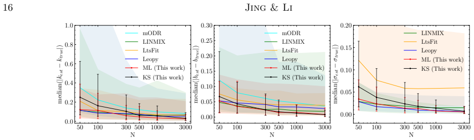
The central claim is that the bias that plagues regression with noisy independent variables can be removed by learning the nuisance distributions from the data itself rather than assuming them. Specifically, the paper argues that a normalizing flow trained on the observed pairs $(x_{\rm obs}, x_{\rm err})$ can recover the latent intrinsic distribution $P(x)$ and the conditional error-level distribution $P(x_{\rm err}|x)$ through the empirical-Bayes marginal likelihood in Eq. (9); plugging these estimates into the full likelihood of Eq. (3) then yields maximum-likelihood estimates of the slope $k$, intercept $b$, and intrinsic scatter $\sigma$ that are unbiased for log-linear relations, provided the sample is large enough (roughly $N>1000$). The KS-test variant replaces the likelihood objective with the p-value of a 2D KS test between data generated by the model and the observed data, and is claimed to be markedly more robust when the model assumptions are violated. The paper further claims that for $300\lesssim N\lesssim 1000$ the ML variant remains the best performer, while for $N<300$ it is competitive with, though no better than, LINMIX and Leopy.

Load-bearing premise

The load-bearing premise is that the normalizing flow trained on observed $(x_{\rm obs},x_{\rm err})$ pairs gives an accurate estimate of the latent intrinsic distribution $P(x)$ and the conditional error distribution $P(x_{\rm err}|x)$, and that these estimates can be treated as known when the regression likelihood is evaluated; if the flow is undertrained or too rigid, the likelihood is misspecified and the regression parameters can be biased, which is consistent with the paper's finding that the advantage shrinks below about 300 samples.

Editorial extensions

If this is right

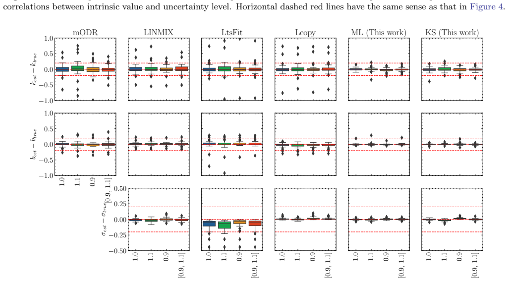
At sample sizes above about 1000, the method is claimed to outperform all eight comparison methods on mock log-linear data, with the KS variant recording an extreme-error fraction of zero for slope, intercept, and scatter across 200 mock datasets.
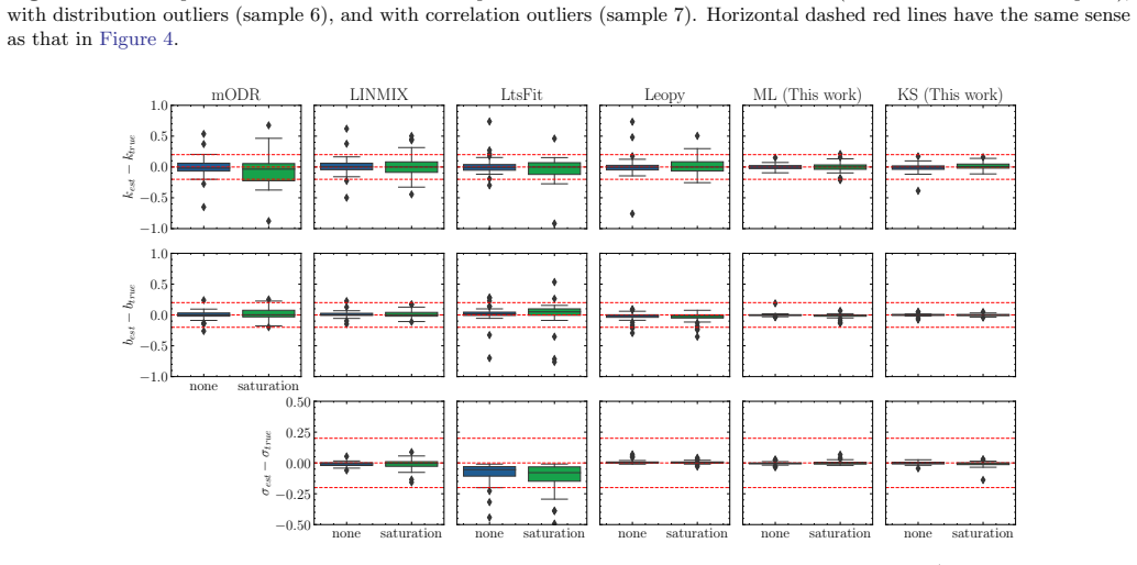
The KS variant is claimed to be robust to violations of the log-linear assumption, complex intrinsic distributions, complex uncertainty-intrinsic correlations, misestimated uncertainties, outliers, and saturation, so it can be applied where standard methods degrade.
For samples of roughly 300–1000, the ML variant is claimed to retain the best median absolute errors, making it the recommended choice in that regime.
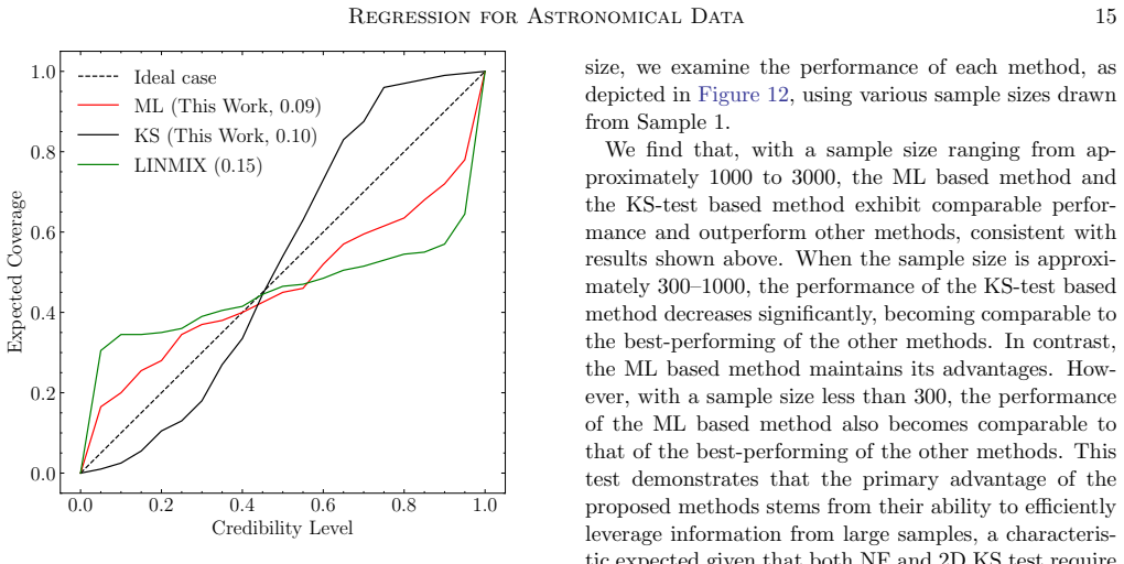
The posterior uncertainties from the new methods are closer to calibrated than LINMIX's (coverage-area 0.09 and 0.10 vs 0.15), though all three remain imperfect.
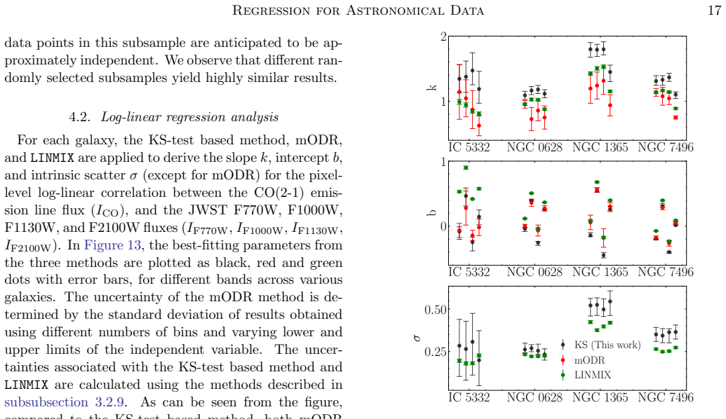
On PHANGS-ALMA and PHANGS-JWST maps of CO(2-1) versus mid-infrared flux, the KS method gives steeper slopes and smaller intercepts than mODR and LINMIX, differences the paper traces to saturation at high flux, noise in the independent variable, and the log-linear versus linear error model.

Reading between the lines

Editorial extensions of the paper, not claims the author makes directly.

Editorial inference: the two-step empirical-Bayes design means the quality of the regression is gated by the quality of the normalizing-flow fit; the paper's own sample-size results are consistent with this, so a practical prescription would be to require a goodness-of-fit check on the flow before trusting the regression output.
Editorial inference: because the likelihood in Eq. (3) is written for a multidimensional independent variable and normalizing flows scale to high dimensions, the same machinery should extend to bivariate or multivariate scaling relations, where Gaussian-mixture-based methods struggle.
Editorial inference: the KS objective, being a distribution-distance criterion, could be reused outside regression — for example, to fit parameters of physical models to noisy observations in other domains where likelihoods are misspecified.
Editorial inference: when $N<300$, the method's advantage disappears; a user with a small sample might do just as well with a simpler method, and a hybrid that injects prior knowledge of $P(x)$ into the flow could extend the regime.

Share X Bluesky LinkedIn Reddit HN

Signed reviews

No signed human review yet.

Editorial analysis

A structured set of objections, weighed in public.

Desk editor's note, referee report, and a circularity audit.

Desk Editor's Note

read the letter

Two things to know. First, this is a real methods paper, not a repackaging: it replaces GMMs or user-supplied P(x) with a normalizing flow estimated from the data, and it models P(x_err|x), which most tools ignore. The mock tests are the strongest part. Second, the central low-S/N claim rests on an empirical-Bayes step that is never directly validated, and the code isn't public yet. Both are fixable.

The likelihood derivation is standard but competently extended. The test suite is broad: 13 intrinsic distributions, several noise models, outliers, saturation, sample-size scaling. Results are consistent, and the KS variant's robustness is impressive. The coverage analysis is a nice touch. They also cite prior work explicitly and correctly.

The latent NF issue is the one that matters. Equations 8-9 estimate P(x) and P(x_err|x) from (x_obs, x_err); the only check is a 2D KS on observables. That does not certify the latent decomposition. In mocks the method does well across many P(x), which is reassuring, but the paper doesn't show recovered versus true P(x) or isolate the NF contribution. Since the headline advantage is at low S/N where these nuisance terms matter most, a referee should ask for that test. Minor: the 2D KS objective is heuristic, the posterior approximation for KS is approximate (they say so), and manual tuning of NF hyperparameters in more than 5% of datasets is a reproducibility concern. Also, a methods paper should not leave the code to acceptance; a public release with a reproducibility script would clear up a lot.

Bottom line: this deserves a serious referee. The contribution is solid and the weaknesses are fixable. I'd ask for code release, a latent-recovery validation on mocks, and a clearer statement of when the KS method's grid search is reliable.

Referee Report

3 major / 4 minor

Summary. The paper proposes two regression methods for astronomical data with measurement errors in both variables, an unknown intrinsic distribution of the independent variable, and correlations between uncertainty levels and intrinsic values. The ML-based method uses a normalizing flow to estimate these nuisance distributions in an empirical-Bayes step, then maximizes the resulting likelihood. The KS-test based variant replaces the likelihood with a 2D Kolmogorov-Smirnov p-value as the optimization objective. Both are tested on extensive mock data covering nonlinearity, complex intrinsic distributions, outliers, saturation, and inaccurate uncertainties, and are applied to PHANGS-ALMA/JWST CO-MIR flux correlations. The central claim is that for sample sizes above 1000, especially at low signal-to-noise ratios, the new methods outperform several established methods (OLS, WLS, ODR, wODR, mODR, LINMIX, LtsFit, Leopy).

Significance. If validated, the methods address a genuine gap: existing Bayesian regression tools such as LINMIX, ROXY, and t-cup rely on Gaussian mixtures and ignore uncertainty-level correlations, while Leopy requires the intrinsic distribution as user input. The mock evaluation is extensive, uses known ground truth (so the performance evidence is external, not circular), and covers a wide range of realistic failure modes. The paper also includes coverage tests and a clear sample-size-dependent recommendation. The code will be made public upon acceptance. However, the central claim rests on the empirical-Bayes step recovering the latent P(x) and P(x_err|x), and this latent recovery is not directly validated; this is the main risk to the soundness of the proposed methods.

major comments (3)

[Section 2.1, Eqs. (7)-(9)] The likelihood in Eq. (3) treats the NF-estimated P(x; phi_2) and P(x_err|x; phi_1) as known. The only validation reported is a 2D KS test comparing the joint observable distribution (x_obs, x_err) to that generated by the fitted NF. This does not certify that the latent decomposition into P(x) and P(x_err|x) is correct; different latent pairs can lead to the same observable joint distribution, especially when the error distribution is flexible. Since the likelihood and the KS generative model use these latent densities directly, a misspecified NF can bias theta in a way that the observable-only KS test may not detect. I ask the authors to add a direct validation of the recovered latent densities on mocks with known truth, or a sensitivity test in which the NF is intentionally misspecified, to demonstrate that the low-S/N advantage is not an artifact of the empirical-Bayes plug-in.
[Section 3.1] The paper states that in more than 95% of datasets the default NF configuration yields a 2D KS p-value above 3e-3, and that 'for the cases where the 2D KS test fails, we manually tune the NF hyperparameters to pass the test.' This manual tuning introduces researcher degrees of freedom into the reported results; for up to 5% of the datasets the final model is not produced by the default algorithm. Since the headline claims include extreme-error fractions of 0 (Figure 2), the fraction of manually tuned datasets should be reported per sample, and the analysis should be repeated without those datasets to show that the conclusions do not depend on manual intervention.
[Section 2.1] The KS-test based method optimizes the p-value of a 2D KS test, which the authors themselves note 'lacks a rigorous mathematical foundation.' The grid-search adaptation and the use of p-values as posterior weights are heuristic. Given that the KS method is recommended as first choice for N>1000, the paper should provide evidence that this objective is well-behaved: for example, a small simulation showing the p-value surface is unimodal, or that the grid search converges to the same solution from different initial ranges. Without this, it is unclear whether the reported robustness of the KS method is a property of the method or of the particular grid-search implementation.

minor comments (4)

[Section 3.2.1] The definition of the extreme error fraction eta (residuals exceeding 1.0 for k and b, and 0.5 for sigma) first appears only in the Figure 1 caption; it would be helpful to define it in the main text.
[Throughout] There are several typographical issues, e.g., 'T able 1' in Section 2.3, 'with espect to' in Section 4.2, and subject-verb agreement errors ('exhibits' vs. 'exhibit' in Sections 3.2.7 and 3.3).
[Section 4.2] The statement that 'different randomly selected subsamples yield highly similar results' is not quantified; please provide the scatter of the fitted parameters across subsamples.
[Section 3.2.9] The coverage test is only performed on three methods; since the paper emphasizes the KS method's robustness, a coverage test on the other compared methods might be informative, but this is optional.

Circularity Check

0 steps flagged · score 1.0 of 10

No significant circularity: central claims are validated on mock data with known ground truth, and the only self-reference is a non-load-bearing announcement of future work.

full rationale

The paper's derivation chain is self-contained and externally tested. The likelihood (Eq. 3) is a standard marginalization over latent intrinsic values; P(x) and P(x_err|x) are nuisance components estimated from the observed data by empirical Bayes (Eqs. 7-9), while the target parameters theta remain free and are optimized against either the likelihood or the 2D KS distance between generated and observed (x_obs, y_obs). No equation defines theta in terms of the NF fit or vice versa, so there is no self-definitional reduction. The principal performance claims are evaluated on mock samples with known k, b, sigma, so the evidence is external to the fitted values; the real-data section is a case study, not a claim of first-principles prediction. The paper explicitly credits prior derivations of similar likelihood formulas (Kelly 2007; Feldmann 2019; Bartlett & Desmond 2023; Martin & Mortlock 2024), so it is not renaming a known result. The only self-references are announcements of a parallel paper (Jing & Li, in prep.) and a fork of the tarp package, neither of which supports the central argument. The reader's concern that NF-estimated latent distributions may be misspecified is a statistical identifiability and robustness risk, not a circularity: the paper's own Figure 12 and the reported >95% successful-fit rate quantify this risk rather than assuming it away.

Assumptions & free parameters 1 free parameters · 4 assumptions · 0 invented entities

The method introduces no new physical entities. The central machinery is a statistical model whose key free choices are the NF architecture and the assumed functional form of the relation.

free parameters (1)

NF architecture hyperparameters = 2 layers, 16 bins, learning rate 3e-3
Chosen by hand; manual tuning used in cases where 2D KS test fails (>5% of runs), affecting reproducibility and potentially biasing results.

assumptions (4)

domain assumption Data points are independent
Assumed in Section 2.1 footnote 1; required for the product form of the likelihood. Downsampling is used in Section 4.1 to approximate independence, but residual correlations may persist.
domain assumption Measurement errors are Gaussian
The likelihood in Eq. 3 assumes Gaussian errors; non-Gaussian errors are not handled.
ad hoc to paper The normalizing flow can represent the true joint distribution of intrinsic value and error size
The method's accuracy depends on the NF approximation; no guarantee of unbiased estimation, especially at finite sample size.
domain assumption The intrinsic scatter in the y-x relation is Gaussian and independent of x
The model P(y|x, theta) is taken as a log-linear relation with Gaussian scatter in the tests; the method allows other forms but tests are limited.

how reviews work

0 comments

Cite this review

Pith. "Pith review of Regression for Astronomical Data with Realistic Distributions, Errors and Non-linearity." pith.science (2026). https://pith.science/paper/OFBIUB6G

@misc{pith2026241108747,
  author       = {Pith},
  title        = {Pith review of: Regression for Astronomical Data with Realistic Distributions, Errors and Non-linearity},
  year         = {2026},
  howpublished = {\url{https://pith.science/paper/OFBIUB6G}},
  note         = {Machine review of arXiv:2411.08747}
}

read the original abstract

We have developed a new regression technique, the maximum likelihood (ML)-based method and its variant, the KS-test based method, designed to obtain unbiased regression results from typical astronomical data. A normalizing flow model is employed to automatically estimate the unobservable intrinsic distribution of the independent variable as well as the unobservable correlation between uncertainty level and intrinsic value of both independent and dependent variables from the observed data points in a variational inference based empirical Bayes approach. By incorporating these estimated distributions, our method comprehensively accounts for the uncertainties associated with both independent and dependent variables. Our test on both mock data and real astronomical data from PHANGS-ALMA and PHANGS-JWST demonstrates that, given a sufficiently large sample size (> 1000), both the ML-based method and the KS-test based method significantly outperform the existing widely-used methods, particularly in cases of low signal-to-noise ratios. The KS-test based method exhibits remarkable robustness against deviations from underlying assumptions, complex intrinsic distributions, varying correlations between uncertainty levels and intrinsic values, inaccuracies in uncertainty estimations, outliers, and saturation effects. For sample sizes between 300 and 1000, the ML-based method yields the best performance. In the low data regime (< 300), the ML-based method maintains comparable performance to other state-of-the-art methods. A GPU-compatible Python implementation of our methods, nicknamed ``raddest'', will be made publicly available upon acceptance of this paper.

Figures

Figures reproduced from arXiv: 2411.08747 by the authors.

**Figure 1.** The residual distribution of k and b for OLS, WLS, ODR, wODR, and mODR. The black histogram represents the distribution of all datasets in sample 1, while the red and blue histogram represents the distribution of the datasets with intrinsic value higher and lower than zero, separately. The vertical dashed lines show the median value of the distribution with same color. The median of the residuals for the entire data… view at source ↗

**Figure 2.** Same as [PITH_FULL_IMAGE:figures/full_fig_p008_2.png] view at source ↗

**Figure 3.** The median absolute error (MAE) of k (left), b (middle) and σ (right) as functions of typical S/N of xobs (upper) and yobs (lower), obtained using different regression methods as indicated. The error bars for the KS-test based method and ML based method and the shaded regions for the other methods indicate the range from 25% quantile to 75% quantile of the absolute errors within each bin of S/N. intrinsic scatter es… view at source ↗

Figures from the paper (12 more)

**Figure 4.** Figure 4: The boxplots of the residual of estimated parameters within different k2 bins in sample 2. A horizontal dashed red line at zero indicates no bias in the residuals. For reference, we include additional horizontal dashed red lines at +0.2 and -0.2. −1.0 −0.5 0.0 0.5 1.0 …

**Figure 5.** Figure 5: Same as [PITH_FULL_IMAGE:figures/full_fig_p011_5.png]

**Figure 6.** Figure 6: The boxplots of the residual of estimated parameters for datasets from sample 1 and sample 3 with different intrinsic log x distributions. Horizontal dashed red lines have the same sense as that in [PITH_FULL_IMAGE:figures/full_fig_p012_6.png]

**Figure 7.** Figure 7: The boxplots of the residual of estimated parameters for datasets from sample 1 and sample 4 with different correlations between intrinsic value and uncertainty level. Horizontal dashed red lines have the same sense as that in [PITH_FULL_IMAGE:figures/full_fig_p013_7.png]

**Figure 8.** Figure 8: The boxplots of the residual of estimated parameters for datasets with accuracy or inaccuracy observed uncertainty level. In each panel, the first bin contains the first 40 datasets from sample 1, which has accuracy observed uncertainty level. The second and third bins…

**Figure 9.** Figure 9: The boxplots of the residual of estimated parameters for datasets without outliers (first 40 datasets from sample 1), with distribution outliers (sample 6), and with correlation outliers (sample 7). Horizontal dashed red lines have the same sense as that in [PITH_FULL…

**Figure 10.** Figure 10: The boxplots of the residual of estimated parameters for datasets without saturation effect (first 40 datasets from sample 1), and datasets with saturation effect (sample 8). Horizontal dashed red lines have the same sense as that in [PITH_FULL_IMAGE:figures/full_fig…

**Figure 11.** Figure 11: Coverage test for KS-test based method, ML based method, and LINMIX. on tarp8 (Lemos et al. 2023) across three methods implemented within a Bayesian or approximate Bayesian framework in our numerical experiments: LINMIX, ML based method, and KS-test based method. For…

**Figure 12.** Figure 12: Same as [PITH_FULL_IMAGE:figures/full_fig_p016_12.png]

**Figure 13.** Figure 13: The best-fitting parameters k, b and σ (alongside their 1σ uncertainties represented as error bars) of the log-linear correlation between the CO(2-1) flux and the mid-infrared fluxes at four JWST bands (F770W, F1000W, F1130W, and F2100W, ordered from left to right fo…

**Figure 14.** Figure 14: In the first row, the distribution of all data points are shown as the black contours. The blue, red, and green contours represent the distribution of mock data points generated based on the best-fitting log-linear relationship obtained by KS-test based method, mODR,…

**Figure 15.** Figure 15: The logarithm of median CO(2-1) flux in each F2100W flux bin for each galaxy is shown as black dots with error bar (for real data, error bar represents 1σ uncertainty of median) and blue dots (for mock data generated by the bestfitting results of KS-test based method…

Discussion (0). Continue with ORCID to comment.

Forward citations

Cited by 1 Pith paper

Reviewed papers in the Pith corpus that reference this work. Sorted by Pith novelty score. Full citation record

The first exploration of the correlations between \textit{WISE} 12 \micron\ and CO emission in early-type galaxies
astro-ph.GA 2024-12 conditional novelty 6.0 of 10

CO luminosity and WISE 12 micron luminosity are tightly correlated in early-type galaxies, with steeper slopes and a constant CO(2-1)-to-CO(1-0) ratio.

Reference graph

Works this paper leans on

26 extracted references · 2 canonical work pages · cited by 1 Pith paper

[1]

, " * write output.state after.block = add.period write newline

ENTRY address archivePrefix author booktitle chapter doi edition editor eprint howpublished institution journal key month number organization pages publisher school series title misctitle type volume year version url label extra.label sort.label short.list INTEGERS output.state before.all mid.sentence after.sentence after.block FUNCTION init.state.consts ...
[2]

write newline

" write newline "" before.all 'output.state := FUNCTION format.url url empty "" new.block "" url * "" * if FUNCTION format.eprint eprint empty "" archivePrefix empty "" archivePrefix "arXiv" = new.block " " eprint * " " * new.block " " eprint * " " * if if if FUNCTION format.doi doi empty "" " " doi * " " * if FUNCTION format.pid doi empty eprint empty ur...
[3]

5B! 5dw.DA2 8-ޛH Z

thebibliography [1] 20pt to REFERENCES 6pt =0pt -12pt 10pt plus 3pt =0pt =0pt =1pt plus 1pt =0pt =0pt -12pt =13pt plus 1pt =20pt =13pt plus 1pt \@M =10000 =-1.0em =0pt =0pt 0pt =0pt =1.0em @enumiv\@empty 10000 10000 `\.\@m \@noitemerr \@latex@warning Empty `thebibliography' environment \@ifnextchar \@reference \@latexerr Missing key on reference command E...

work page arXiv 2021
[4]

G., & Bershady , M

Akritas , M. G., & Bershady , M. A. 1996, , 470, 706, 10.1086/177901

doi:10.1086/177901 1996
[5]

J., & Desmond , H

Bartlett , D. J., & Desmond , H. 2023, The Open Journal of Astrophysics, 6, 42, 10.21105/astro.2309.00948

arXiv 2023
[6]

2013, MNRAS, 432, 1709, 10.1093/mnras/stt562

Cappellari , M., Scott , N., Alatalo , K., et al. 2013, MNRAS, 432, 1709, 10.1093/mnras/stt562

doi:10.1093/mnras/stt562 2013
[7]

K., Sandstrom , K., et al

Chown , R., Leroy , A. K., Sandstrom , K., et al. 2024, arXiv e-prints, arXiv:2410.05397, 10.48550/arXiv.2410.05397

arXiv doi:10.48550/arxiv.2410.05397 2024
[8]

F., Kalmbach, J

Crenshaw, J. F., Kalmbach, J. B., Gagliano, A., et al. 2024 a , Probabilistic Forward Modeling of Galaxy Catalogs with Normalizing Flows. 2405.04740

arXiv 2024

Show all 26 references

[9]

F., Yan, Z., & Doster, V

Crenshaw, J. F., Yan, Z., & Doster, V. 2024 b , jfcrenshaw/pzflow: v3.1.3, v3.1.3, Zenodo, 10.5281/zenodo.10710271

2024 doi
[10]

2014, arXiv e-prints, arXiv:1410.8516, 10.48550/arXiv.1410.8516

Dinh , L., Krueger , D., & Bengio , Y. 2014, arXiv e-prints, arXiv:1410.8516, 10.48550/arXiv.1410.8516

2014 doi arXiv
[11]

L., Lin , L., Thorp , M

Ellison , S. L., Lin , L., Thorp , M. D., et al. 2021, , 501, 4777, 10.1093/mnras/staa3822

2021 doi
[12]

2019, Astronomy and Computing, 29, 100331, 10.1016/j.ascom.2019.100331

Feldmann , R. 2019, Astronomy and Computing, 29, 100331, 10.1016/j.ascom.2019.100331

2019
[13]

Fuller, W. A. 2009, Measurement error models (John Wiley & Sons)

2009
[14]

W., Bovy , J., & Lang , D

Hogg , D. W., Bovy , J., & Lang , D. 2010, arXiv e-prints, arXiv:1008.4686, 10.48550/arXiv.1008.4686

2010 doi arXiv
[15]

D., Akritas , M

Isobe , T., Feigelson , E. D., Akritas , M. G., & Babu , G. J. 1990, , 364, 104, 10.1086/169390

1990 doi
[16]

2015, arXiv e-prints, arXiv:1505.05770, 10.48550/arXiv.1505.05770

Jimenez Rezende , D., & Mohamed , S. 2015, arXiv e-prints, arXiv:1505.05770, 10.48550/arXiv.1505.05770

2015 doi arXiv
[17]

Kelly , B. C. 2007, , 665, 1489, 10.1086/519947

2007 doi
[18]

2021, Research Notes of the American Astronomical Society, 5, 39, 10.3847/2515-5172/abe8df

Klein , R. 2021, Research Notes of the American Astronomical Society, 5, 39, 10.3847/2515-5172/abe8df

2021 doi
[19]

C., Sandstrom , K

Lee , J. C., Sandstrom , K. M., Leroy , A. K., et al. 2023, , 944, L17, 10.3847/2041-8213/acaaae

2023 doi
[20]

K., Hughes , A., Liu , D., et al

Leroy , A. K., Hughes , A., Liu , D., et al. 2021 a , , 255, 19, 10.3847/1538-4365/abec80

2021 doi
[21]

K., Schinnerer , E., Hughes , A., et al

Leroy , A. K., Schinnerer , E., Hughes , A., et al. 2021 b , , 257, 43, 10.3847/1538-4365/ac17f3

2021 doi
[22]

K., Sandstrom , K., Rosolowsky , E., et al

Leroy , A. K., Sandstrom , K., Rosolowsky , E., et al. 2023, , 944, L9, 10.3847/2041-8213/acaf85

2023 doi
[23]

Peacock , J. A. 1983, , 202, 615, 10.1093/mnras/202.3.615

1983 doi
[24]

H., Teukolsky , S

Press , W. H., Teukolsky , S. A., Vetterling , W. T., & Flannery , B. P. 1992, Numerical recipes in FORTRAN. The art of scientific computing

1992
[25]

Robotham , A. S. G., & Obreschkow , D. 2015, , 32, e033, 10.1017/pasa.2015.33

2015 doi
[26]

G., Lee , J

Williams , T. G., Lee , J. C., Larson , K. L., et al. 2024, , 273, 13, 10.3847/1538-4365/ad4be5

2024 doi

Pith tools

Reviewed August 12, 2026 · model on record in the stance chip above.

[1] [1]

, " * write output.state after.block = add.period write newline

ENTRY address archivePrefix author booktitle chapter doi edition editor eprint howpublished institution journal key month number organization pages publisher school series title misctitle type volume year version url label extra.label sort.label short.list INTEGERS output.state before.all mid.sentence after.sentence after.block FUNCTION init.state.consts ...

[2] [2]

write newline

" write newline "" before.all 'output.state := FUNCTION format.url url empty "" new.block "" url * "" * if FUNCTION format.eprint eprint empty "" archivePrefix empty "" archivePrefix "arXiv" = new.block " " eprint * " " * new.block " " eprint * " " * if if if FUNCTION format.doi doi empty "" " " doi * " " * if FUNCTION format.pid doi empty eprint empty ur...

[3] [3]

5B! 5dw.DA2 8-ޛH Z

thebibliography [1] 20pt to REFERENCES 6pt =0pt -12pt 10pt plus 3pt =0pt =0pt =1pt plus 1pt =0pt =0pt -12pt =13pt plus 1pt =20pt =13pt plus 1pt \@M =10000 =-1.0em =0pt =0pt 0pt =0pt =1.0em @enumiv\@empty 10000 10000 `\.\@m \@noitemerr \@latex@warning Empty `thebibliography' environment \@ifnextchar \@reference \@latexerr Missing key on reference command E...

work page arXiv 2021

[4] [4]

G., & Bershady , M

Akritas , M. G., & Bershady , M. A. 1996, , 470, 706, 10.1086/177901

doi:10.1086/177901 1996

[5] [5]

J., & Desmond , H

Bartlett , D. J., & Desmond , H. 2023, The Open Journal of Astrophysics, 6, 42, 10.21105/astro.2309.00948

arXiv 2023

[6] [6]

2013, MNRAS, 432, 1709, 10.1093/mnras/stt562

Cappellari , M., Scott , N., Alatalo , K., et al. 2013, MNRAS, 432, 1709, 10.1093/mnras/stt562

doi:10.1093/mnras/stt562 2013

[7] [7]

K., Sandstrom , K., et al

Chown , R., Leroy , A. K., Sandstrom , K., et al. 2024, arXiv e-prints, arXiv:2410.05397, 10.48550/arXiv.2410.05397

arXiv doi:10.48550/arxiv.2410.05397 2024

[8] [8]

F., Kalmbach, J

Crenshaw, J. F., Kalmbach, J. B., Gagliano, A., et al. 2024 a , Probabilistic Forward Modeling of Galaxy Catalogs with Normalizing Flows. 2405.04740

arXiv 2024