Optimal Transport-Based Displacement Interpolation with Data Augmentation for Reduced Order Modeling of Nonlinear Dynamical Systems

Annalisa Quaini; Federico Pichi; Gianluigi Rozza; Michele Girfoglio; Moaad Khamlich

REVIEW 4 major objections 4 minor 67 references

Optimal Transport-Based Displacement Interpolation with Data Augmentation for Reduced Order Modeling of Nonlinear Dynamical Systems

T0 review · 4 major / 4 minor · reviewed 2026-08-12 · deepseek-v4-flash

Challenge this review Re-run · record.json Download PDF Read on arXiv ↗ Review JSON

Pith's one-line read The paper claims that displacement interpolation along optimal-transport geodesics between checkpoint snapshots generates physically consistent synthetic data that, combined with a virtual-to-real time mapping and a Gaussian-process…

desk verdict A useful, honest OT-based data augmentation ROM with coherent error trends, but the improved-accuracy claim needs a proper no-OT baseline and the transport assumption only holds with dense checkpoints. read the letter →

arxiv 2411.08750 v1 pith:HOGGK4FN submitted 2024-11-13 math.NA cs.LGcs.NA

Moaad Khamlich , Federico Pichi , Michele Girfoglio , Annalisa Quaini , Gianluigi Rozza This is my paper · ORCID

classification math.NAcs.LGcs.NA MSC 49Q2265M08

keywords Reduced-ordermodelsOptimaltransportDisplacementinterpolationWassersteindistanceDataaugmentationGaussianprocessregressionAtmosphericflowsimulationAdvection-dominateddynamics

verification ladder T0 review T1 audit T2 compute T3 formal

The pith

A machine-rendered reading of the paper's core claim, the machinery that carries it, and where it could break.

The reading

This paper proposes that optimal transport's displacement interpolation—the geodesic path between two probability measures in Wasserstein space—can generate synthetic solution snapshots for training reduced-order models of nonlinear, advection-dominated PDEs. The authors' claim is that interpolating between selected checkpoints along these geodesics yields intermediate states that are physically consistent enough to enrich a POD basis, allowing accurate predictions at arbitrary times even when only coarse and sparse training data are available. They add a virtual-to-real time mapping to attach physical time labels to the synthetic snapshots, and a Gaussian-process regression correction that learns the residual between the interpolated states and the true solution. On two atmospheric benchmarks, a rising thermal bubble and a density current, the method is shown to reduce interpolation and generalization errors and to deliver online speed-ups of roughly two orders of magnitude relative to the full-order solver.

What carries the argument

The workhorse is displacement interpolation between probability measures, defined in Eq. (14): given an optimal transport plan $\pi_\epsilon$ between two checkpoints, the intermediate state at virtual time $\alpha$ is $\left((1-\alpha)\|u_{k_i}\|_1 + \alpha\|u_{k_{i+1}}\|_1\right)\sum_{l,m}(\pi_\epsilon)_{lm}\delta_{\mathrm{proj}_X((1-\alpha)x_l+\alpha x_m)}$, with positive and negative parts of the field interpolated separately when the field changes sign. The entropic regularization of the transport plan in Eq. (13) makes the plan computable by Sinkhorn-type iterations while remaining close to a true geodesic. Two auxiliary mechanisms carry the online phase: a virtual-to-real time map $F\in\{L,M\}$, where $L$ is piecewise linear and $M$ is a least-squares regression of the global interpolation parameter against physical time, and a POD/GPR residual corrector in Eqs. (21)–(23) that predicts the POD coefficients of the bias $\mathbf{r}_k = u^k_h - u_{\mathrm{synth}}(F_1(t_k),F_2(t_k))$.

What would settle it

Run a pair of consecutive checkpoints that straddle a feature which rotates in place or diffuses symmetrically (for example, a stationary diffusing Gaussian bump or a vortex dipole), compute the displacement-interpolated midpoint at $\alpha=1/2$, and compare it with the full-order solution at the corresponding physical time; the transport-only hypothesis is what fails if the midpoint error remains far above the time-discretization error and the POD/GPR correction cannot close the gap.

Watch

Extended reading notes

Core claim

The central discovery is that the slow decay of the Kolmogorov n-width that plagues linear ROMs for advection-dominated problems can be partially circumvented at the data level: instead of approximating the solution manifold only with a linear subspace of snapshots, one enriches the snapshot set with displacement interpolants that trace Wasserstein geodesics between checkpoints. For scalar fields the method splits the field into positive and negative parts, normalizes each to unit mass, solves the entropically regularized optimal transport problem between consecutive checkpoints, and pushes each mass particle along a straight line per Eq. (14), with a mass-interpolation factor and a projection back to the computational grid. The paper argues these synthetic snapshots capture genuinely transported features—fronts, rising bubbles, cold-air lobes—so the resulting POD basis is more expressive per mode than one built from checkpoints alone. The residual between geodesic interpolation and the true trajectory is then modeled by POD with Gaussian process regression, which the paper presents as the component that recovers fine-scale structures such as Kelvin–Helmholtz billows.

Load-bearing premise

The load-bearing premise is that the physics between two chosen checkpoints is, to first order, pure mass transport: every feature at the later checkpoint can be obtained by moving the features at the earlier one along straight lines, with no significant creation, destruction, diffusion, or rotation in between.

Editorial extensions

If this is right

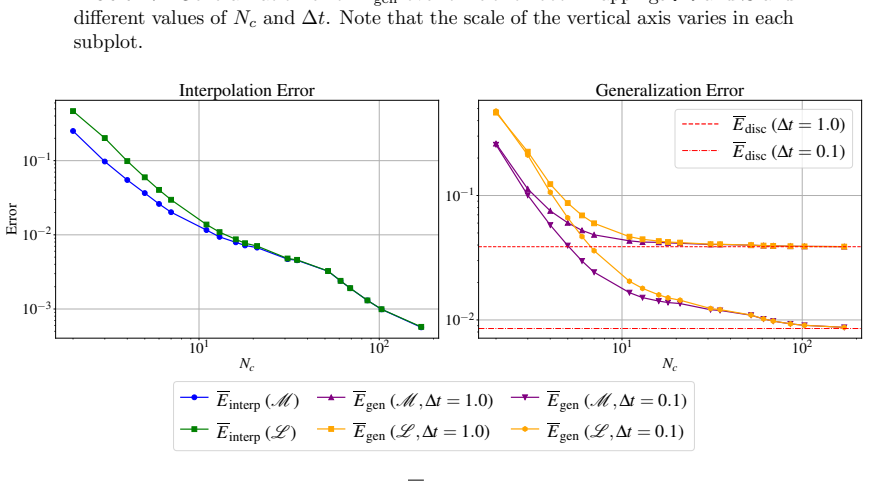
As the number of checkpoints $N_c$ grows, the interpolation error decreases monotonically and the generalization error saturates at the time-discretization error of the training data, so the method cannot beat the temporal resolution of the data it is trained on.
The optimal regression map $M$ is more accurate than the linear map $L$ when the solution's rate of change is non-uniform, and the two coincide as $N_c$ increases.
A POD basis built from synthetic OT snapshots has lower projection error than a basis built from checkpoints alone, especially when checkpoints are few and the training time step is coarse.
The POD+GPR residual correction reduces both interpolation and generalization errors in the density current test, with the largest gains when few checkpoints are used, and is what recovers fine-scale Kelvin–Helmholtz structures.
Online inference at arbitrary times costs a matrix-vector multiplication with precomputed plans and achieves speed-ups of order $10^2$ over the reference full-order simulation.

Reading between the lines

Editorial extensions of the paper, not claims the author makes directly.

Implicit extension: the data augmentation step is separable from the rest of the pipeline, so any non-intrusive ROM—including neural-network regressors that need large training sets—could consume the synthetic snapshot matrix $S_{\mathrm{synth}}$ directly.
The transport-only assumption suggests the method should transfer well to Lagrangian or interface-tracking formulations, but it also predicts failure modes: checkpoint intervals containing significant diffusion, chemical reaction, or vortex rotation would need denser checkpoints or an extra non-transport correction.
An adaptive checkpoint selection rule driven by the OT cost between adjacent snapshots, or by a local estimate of the Wasserstein distance traveled, is a natural extension that could reduce the number of checkpoints needed on intervals where the solution barely changes.
If the MinL2 map $M$ is interpreted as a learned time-warping, the same construction could be used for temporal super-resolution of experimental image sequences such as PIV data, where no full-order model exists.

Share X Bluesky LinkedIn Reddit HN

Signed reviews

No signed human review yet.

Editorial analysis

A structured set of objections, weighed in public.

Desk editor's note, referee report, and a circularity audit.

Desk Editor's Note

read the letter

Short version: this is a useful, honest engineering paper, not a breakthrough. The pipeline is sensible and the reported error behavior is coherent — Egen drops as Nc grows and saturates at Edisc, and the synthetic POD basis beats the checkpoint-only basis. The main gap is that the paper never runs the natural control experiment: the same POD-R pipeline without the OT augmentation. Without that, the headline "improved accuracy" is asserted rather than demonstrated.

What is genuinely new: previous displacement-interpolation ROM work (Iollo/Taddei, Cucchiara et al.) was restricted to Gaussian OT maps. Here the entropic OT plan is computed directly on the discrete fields, with positive/negative splitting, checkpoint intervals, a virtual-to-real time mapping (linear and MinL2), and a GPR residual correction. That combination is new, and the modular design means the data augmentation part can be reused by other non-intrusive ROMs.

The experiments are mostly well done. The two atmospheric benchmarks are appropriate. The observation that Egen saturates at the time discretization error is a good sanity check. The speed-up figures are honest — online inference is cheap, offline OT solves dominate but are parallelizable. The authors also deserve credit for explicitly noting that Nc=2 gives a physically irrelevant trajectory (Figure 4) and for being upfront about it.

The soft spots are real but not fatal. First, no end-to-end baseline: the POD-basis comparison is not the same as showing the full ROM is more accurate than a POD-R without OT. Second, key implementation details are missing — epsilon for the entropic OT, GPR hyperparameters, and exactly how the signed-field split is done (threshold, handling of zeros). Third, the load-bearing transport assumption is not validated directly. For the thermal bubble and density current, the dynamics include vortical roll-up and diffusion, so the quadratic-cost OT plan is not the physical flow map. The paper recovers by choosing enough checkpoints, which is reasonable, but it means the synthetic snapshots are better described as geometrically plausible intermediates than as physically consistent states. The independent transport of positive and negative anomalies can also allow unphysical crossing, though the error metrics suggest the practical impact is limited. The residual correction presumably hides some of this, but the paper doesn't quantify how much.

Who should read it: people working on non-intrusive ROMs for advection-dominated problems and anyone thinking about data augmentation for limited-data ROM training. It deserves peer review. The referee should ask for the no-OT baseline, full parameter tables, and ideally code/data release.

Referee Report

4 major / 4 minor

Summary. The manuscript presents a reduced-order modeling framework for time-dependent nonlinear advection-dominated PDEs. From a set of Nc checkpoint snapshots, the authors compute entropically regularized optimal transport plans between consecutive checkpoints and use displacement interpolation (Eq. 14) to synthesize Nsynth intermediate snapshots per interval. A virtual-to-real time mapping (piecewise linear L or regression-based M) labels the synthetic snapshots with physical time, and a POD+GPR correction (Eqs. 22-23) is added to reduce residual bias. The method is applied to the rising thermal bubble and the density current benchmarks for mesoscale atmospheric flow, with θ' as the field of interest. Reported results show that mean interpolation and generalization errors decrease as Nc increases and saturate near the training time-discretization error Edisc, that the MinL2 mapping M outperforms the linear mapping L for small Nc, that POD bases from synthetic data give lower projection errors than checkpoint-only bases, and that the POD correction improves density-current errors.

Significance. The framework addresses a real limitation of linear ROMs for advection-dominated problems, and the error decomposition into Edisc, Einterp, and Egen is a useful methodological contribution. The paper also provides a falsifiable prediction: Egen should saturate at Edisc as Nc grows. The use of open-source software (GEA, MultiScaleOT) and the reporting of computational timings and speed-ups are strengths. However, the evidence for the headline claim of 'improved accuracy' is incomplete: the paper does not compare the full pipeline against a standard ROM without OT augmentation, and the physical consistency of the displacement interpolation is validated only indirectly and only for sufficiently short checkpoint intervals. These gaps make the current version a solid proof-of-concept rather than a fully supported general method.

major comments (4)

[Section 6, Figures 8-9] The central claim of improved ROM accuracy is not supported by an end-to-end comparison against a standard non-intrusive ROM without OT augmentation. Figures 8 and 9 quantify the interpolation/generalization error of the OT surrogate itself and the projection error of POD bases built from Ssynth versus Scheck, and Figure 14 shows the effect of the POD correction only for the density current. Missing is a comparison, under identical training and test data, between the complete pipeline in Eq. (23) and a baseline such as POD-R trained on the Nc checkpoints only, or POD-R trained on the original Ntrain snapshots with piecewise-linear time interpolation. Without that baseline, the reported gains could be attributed to the larger number of snapshots in Ssynth rather than to the OT displacement structure.
[Section 4, Steps (2)-(3) and Eq. (14)] The construction of synthetic snapshots for signed fields is under-specified. The text says that for θ' the positive and negative parts are normalized and transported separately, but it never states how the two independently transported components are recombined into usynth in Eq. (14). Because the two OT plans are independent, positive and negative anomalies can be transported along different paths and overlap in unphysical ways; the paper should specify the recombination and provide a direct check that intermediate fields satisfy basic consistency conditions, such as reproducing the checkpoints at α=0,1 and not creating spurious extrema beyond the entropy-regularization blurring.
[Section 4, Step (3); Figure 4; Remark 4.2] The physical-consistency assumption behind displacement interpolation is only demonstrated in the limit of short checkpoint intervals. The paper itself describes the Nc=2 trajectory in Figure 4 as 'of limited physical relevance,' and Egen in Figures 7-8 is large until Nc is large enough that the interval length is small. This success for large Nc is consistent with any interpolation scheme becoming accurate on short intervals, so it does not specifically validate the Wasserstein-geodesic model. Please quantify the checkpoint interval Δtc at which Egen reaches Edisc and, for at least one interval, compare the OT displacement plan with the physical flow map obtained from the velocity field.
[Section 6.2, Figure 14] The POD-based correction (Eqs. 22-23) is a key component of the framework, but results are reported only for the density current. For the thermal bubble, no corrected Egen or Einterp curves are shown, despite the text stating that the correction 'consistently reduces the error.' Please add the corrected-error curves for the thermal bubble, or state explicitly that the correction was not applied in that benchmark.

minor comments (4)

[Section 2.1, Eq. (3)] The POD minimization should include the orthogonality constraint U^T U = I; as written, the argmin over all matrices in R^{Nh×Nr} is not the standard POD problem and admits non-unique solutions.
[Section 4, Eq. (14)] The formula for usynth uses the L1 norm on the checkpoint fields before normalization, but the OT plan in Eq. (13) is computed between normalized measures; the relation between those normalizations and the mass-interpolation factor (A) should be made explicit, especially for the positive/negative split.
[Section 6.1, definition of Ttest] The expression Ttest = {j + (0.05 ± Δttest) | j=1,...,NT} is ambiguous; please write the two test-point sets explicitly.
[Figure 2] Figure 2 is referenced as a schematic of the methodology but is not described in the text; adding a short explanation of the data flow would improve readability.

Circularity Check

0 steps flagged · score 1.0 of 10

No significant circularity: OT plans, time-to-alpha mappings, and GPR residual corrections are all built from coarse training snapshots only, and the headline accuracy claims are validated against external fine-reference test snapshots; only a minor non-load-bearing self-citation and a transparently labeled training-fit metric keep the score slightly above zero.

full rationale

No significant circularity. The predictive claims rest on the generalization error Egen (Eq. 44), which compares the synthetic reconstruction usynth(F(t*)) at test times t* in Ttest against the fine-reference solution theta'_ref(t*) computed with Delta t_ref = 0.005 s (Sec. 6). The OT plans (Eq. 13) use only checkpoints drawn from the coarse training trajectory Sh; the MinL2 virtual-to-real mapping M is fit only on training pairs {(tk, alpha_global,k)} (Eq. 19); and the POD-R/GPR residual correction (Eqs. 22-23) is trained only on residuals rk = u^k_h - usynth(F1(tk), F2(tk)) at training times. Ttest is defined to have no intersection with Ttrain, so no test snapshot enters any of these fits; hence the central claim does not reduce to its inputs by construction. Two near-misses are weighed but do not rise to circularity. First, Einterp(M) (Eq. 43) is by construction the normalized training objective that M minimizes in Eqs. (18)-(19), so M's interpolation-error advantage over L is a fit artifact; however, the paper explicitly labels Einterp as the error on training data ('The interpolation error quantifies the accuracy of our synthetic snapshots interpolating the training data') and bases its predictive claims on Egen, which uses external fine-reference data. Second, reference [36] is the present authors' own prior work, cited only as contextual related work on Wasserstein-kernel kPOD; it is not load-bearing, and the OT machinery itself cites external theory (McCann, Villani, Santambrogio, Cuturi, Schmitzer). The paper also concedes in Section 6.1 and Figure 4 that the transport assumption yields trajectories of limited physical relevance for Nc = 2, i.e., the central modeling assumption is empirically exposed to falsification rather than enforced by definition. Honest finding: score 1 reflects the minor self-citation and the training-fit metric, not substantive circularity.

Assumptions & free parameters 6 free parameters · 5 assumptions · 0 invented entities

The central claim rests on standard OT/POD machinery, a transport-dominance modeling assumption, and several unreported hyperparameters. No new physical entities are introduced.

free parameters (6)

Number of checkpoints Nc = varied: 2, 11, 31, 61, 103, 171 (bubble); 2, 11, 31, 151 (density current)
User-selected hyperparameter; strongly controls OT computation cost and interpolation fidelity.
Entropic regularization epsilon = not reported
Controls Sinkhorn plan smoothness in Eq. (13) and is never specified in the manuscript.
Synthetic snapshots per interval Nsynth = floor((Ntot-Nc)/(Nc-1)) with Ntot=1021
Determines the density of augmented snapshots; tied to Nc rather than optimized.
POD energy threshold for residual basis = 99.99%
Sets the number of residual modes in the POD correction step; no sensitivity study is given.
GPR hyperparameters = not reported
Kernel, length scales, and noise parameters for the Gaussian process in Eq. (22) are not given.
Artificial viscosity and Prandtl number = mu_a=15, Pr=1 (bubble); mu_a=75, Pr=1 (density current)
Chosen ad hoc (stated in Section 6.1) to stabilize the full-order benchmark; they shape the reference data.

assumptions (5)

standard math Optimal transport, Sinkhorn algorithm, POD/SVD, and Gaussian process regression are valid background tools.
Invoked in Sections 2-4 without proof; standard literature is cited.
domain assumption A discretized scalar field can be split into positive and negative parts, normalized, and treated as probability measures for OT.
Section 4, Step 2; no proof that this preserves the physical interpretation under displacement interpolation.
domain assumption The field evolution between checkpoints is transport-dominated, so straight-line displacement interpolation in Wasserstein space yields states close to the true solution.
Section 4, Step 3 and Eq. (14); the central modeling premise, only indirectly validated by error metrics.
domain assumption Coarse training data define an error floor Edisc, and the ROM cannot be expected to beat that floor.
Section 6 error definitions; used to interpret saturation of Egen.
ad hoc to paper Checkpoints are chosen as a uniform subset and the MinL2 mapping is fit to training snapshots.
Section 4, Step 4; both choices are method design decisions not derived from physical or mathematical constraints.

how reviews work

0 comments

Cite this review

Pith. "Pith review of Optimal Transport-Based Displacement Interpolation with Data Augmentation for Reduced Order Modeling of Nonlinear Dynamical Systems." pith.science (2026). https://pith.science/paper/HOGGK4FN

@misc{pith2026241108750,
  author       = {Pith},
  title        = {Pith review of: Optimal Transport-Based Displacement Interpolation with Data Augmentation for Reduced Order Modeling of Nonlinear Dynamical Systems},
  year         = {2026},
  howpublished = {\url{https://pith.science/paper/HOGGK4FN}},
  note         = {Machine review of arXiv:2411.08750}
}

read the original abstract

We present a novel reduced-order Model (ROM) that leverages optimal transport (OT) theory and displacement interpolation to enhance the representation of nonlinear dynamics in complex systems. While traditional ROM techniques face challenges in this scenario, especially when data (i.e., observational snapshots) is limited, our method addresses these issues by introducing a data augmentation strategy based on OT principles. The proposed framework generates interpolated solutions tracing geodesic paths in the space of probability distributions, enriching the training dataset for the ROM. A key feature of our approach is its ability to provide a continuous representation of the solution's dynamics by exploiting a virtual-to-real time mapping. This enables the reconstruction of solutions at finer temporal scales than those provided by the original data. To further improve prediction accuracy, we employ Gaussian Process Regression to learn the residual and correct the representation between the interpolated snapshots and the physical solution. We demonstrate the effectiveness of our methodology with atmospheric mesoscale benchmarks characterized by highly nonlinear, advection-dominated dynamics. Our results show improved accuracy and efficiency in predicting complex system behaviors, indicating the potential of this approach for a wide range of applications in computational physics and engineering.

Figures

Figures reproduced from arXiv: 2411.08750 by the authors.

**Figure 1.** Displacement interpolation between two discrete distributions µ0 and µ1 shown on the left panel. In the right panel, the point’s masses are proportional to the size of the point and OT plan line thickness are proportional to the mass transported. Key properties of displacement interpolation include: (i) geodesicity, as µα traces a geodesic in the Wasserstein space of probability measures; (ii) mass conservation with… view at source ↗

**Figure 2.** Schematic depiction of our OT-based interpolation ROM approach. (3) Synthetic Data Generation: Let X = {xl} Nh l=1 be the set of discretization points in our numerical scheme, shared by all fields. These points represent, for example, cell centroids in a FV discretization. Let α ∈ [0, 1] be the local interpolation parameter, playing the role of virtual time. We define a function usynth(i, α), for i ∈ {0, 1, . . . , … view at source ↗

**Figure 3.** Evolution of the potential temperature perturbation field θ ′ for the rising thermal bubble test case. We impose impenetrable, free-slip boundary conditions on all domain boundaries. The simulation is run for a total time of tf = 1021 s. During this time interval, the warm bubble rises due to buoyancy forces and evolves into a characteristic mushroom-like shape as a result of shear stresses at its edges. See [PITH_… view at source ↗

Figures from the paper (11 more)

**Figure 4.** Figure 4: Evolution of synthetic solutions for the rising thermal bubble as the number of checkpoints Nc varies. The images demonstrate how increasing Nc leads to more physically relevant interpolated trajectories. Number of Checkpoints (Nc) 2 11 31 61 103 171 Step 2-3 (%) 81.74…

**Figure 5.** Figure 5: Speed-up factor as a function of the number of checkpoints Nc for the rising thermal bubble test case. 0 500 1000 t 0.0 0.2 0.4 0.6 0.8 1.0 αglobal ( M ) Nc = 2 0 500 1000 t 0.0 0.2 0.4 0.6 0.8 1.0 αglobal ( M ) Nc = 11 0 500 1000 t 0.0 0.2 0.4 0.6 0.8 1.0 αglobal ( M …

**Figure 6.** Figure 6: Global interpolation parameter αglobal(M) in red and its deviation in blue over time for Nc = 2 (left), Nc = 11 (center), Nc = 171 (right) [PITH_FULL_IMAGE:figures/full_fig_p015_6.png]

**Figure 7.** Figure 7: Generalization error Egen over time t for both mappings M and L and different values of Nc and ∆t. Note that the scale of the vertical axis varies in each subplot. 101 102 Nc 10−3 10−2 10−1 Error Interpolation Error 10 1 10 2 Nc 10−2 10−1 Generalization Error Edisc (∆t…

**Figure 8.** Figure 8: Mean interpolation error Einterp (left) and mean generalization error Egen (right) for both mappings M and L vs. the number of checkpoints Nc for different time step sizes ∆t. POD bases obtained from Ssynth and Scheck, respectively. We compute the projection errors for…

**Figure 9.** Figure 9: presents the projection errors for both Usynth and Ucheck across different values of Nc and ∆t. For ∆t = 1 s, the projection error for Usynth becomes comparable to Edisc with as few as 3 checkpoints, while for ∆t = 0.1 s it takes 11 checkpoints. This difference can be …

**Figure 10.** Figure 10: Evolution of the potential temperature perturbation field θ ′ for the density current test case. Following [62], we set µa = 75 m2 s −1 and Pr = 1. The reference solution uses ∆tref = 0.005 s, while training solutions use ∆ttrain ∈ {0.01 s, 0.1 s}. Unlike the thermal …

**Figure 11.** Figure 11: Evolution of synthetic solutions for the density current as the number of checkpoints Nc varies. 0 250 500 750 t 0.00 0.25 0.50 0.75 1.00 αglobal ( M ) Nc = 2 0 250 500 750 t 0.0 0.2 0.4 0.6 0.8 1.0 αglobal ( M ) Nc = 11 0 250 500 750 t 0.0 0.2 0.4 0.6 0.8 1.0 αglobal…

**Figure 12.** Figure 12: Global interpolation parameter αglobal(M) in red and its deviation in blue over time for Nc = 2 (left), Nc = 11 (center), Nc = 151 (right). for capturing fine-scale structures like Kelvin-Helmholtz instability along the upper boundary of the cold front, which are chal…

**Figure 13.** Figure 13: Generalization error Egen over time t for both mappings M and L and different values of Nc and ∆t. Note that the scale of the vertical axis varies in each subplot. 101 102 Nc 10−3 10−2 10−1 100 Error Interpolation Error 10 1 10 2 Nc 10−2 10−1 100 Generalization Error …

**Figure 14.** Figure 14: Mean interpolation error Einterp (left) and mean generalization error Egen (right) for both mappings M and L vs. the number of checkpoints Nc for different time step sizes ∆t. The goal is to show the effect of the POD-based correction on errors Einterp and Egen. 7. Co…

Discussion (0). Continue with ORCID to comment.

Reference graph

Works this paper leans on

67 extracted references · 37 canonical work pages

[1]

Hager and G

G. Hager and G. Wellein. Introduction to High Performance Computing for Scientists and Engineers. CRC Press, Inc., USA, 1st edition, 2010

work page 2010
[2]

Benner, S

P. Benner, S. Gugercin, and K. Willcox. A survey of projection-based model reduction methods for parametric dynamical systems. SIAM review, 57(4):483–531, 2015. doi:10.1137/130932715

doi:10.1137/130932715 2015
[3]

Benner, A

P. Benner, A. Cohen, M. Ohlberger, and K. Willcox. Model Reduction and Approximation: Theory and Algo- rithms. SIAM, Society for Industrial and Applied Mathematics, 2017. URL https://books.google.it/books? id=hbEsDwAAQBAJ

work page 2017
[4]

M. A. Grepl, Y. Maday, N. C. Nguyen, and A. T. Patera. Efficient reduced-basis treatment of nonaffine and nonlinear partial differential equations. ESAIM: Mathematical Modelling and Numerical Analysis , 41(3):575– 605, 2007. URL http://eudml.org/doc/250042

work page 2007
[5]

Schilders, H

W. Schilders, H. Van der Vorst, and J. Rommes. Model Order Reduction: Theory, Research Aspects and Appli- cations, volume 13. Springer Berlin Heidelberg, 01 2008. doi:10.1007/978-3-540-78841-6

doi:10.1007/978-3-540-78841-6 2008
[6]

Rozza, D

G. Rozza, D. B. P. Huynh, and A. T. Patera. Reduced basis approximation and a posteriori error estimation for affinely parametrized elliptic coercive partial differential equations: Application to transport and continuum mechanics. Archives of Computational Methods in Engineering , 15(3):229–275, May 2008. doi:10.1007/s11831- 008-9019-9

doi:10.1007/s11831- 2008
[7]

Lassila, A

T. Lassila, A. Manzoni, A. Quarteroni, and G. Rozza. Model Order Reduction in Fluid Dynamics: Challenges and Perspectives, pages 235–273. Springer International Publishing, Cham, 2014

work page 2014
[8]

J. S. Hesthaven, G. Rozza, and B. Stamm. Certified Reduced Basis Methods for Parametrized Partial Differential Equations. Springer International Publishing, 2016. doi:10.1007/978-3-319-22470-1

doi:10.1007/978-3-319-22470-1 2016

Show all 67 references

[9]

Quarteroni, A

A. Quarteroni, A. Manzoni, and F. Negri. Reduced Basis Methods for Partial Differential Equations . Springer International Publishing, 2016. doi:10.1007/978-3-319-15431-2

2016 doi
[10]

Benner, S

P. Benner, S. Grivet-Talocia, A. Quarteroni, G. Rozza, W. Schilders, and L. Miguel Silveira. Model Order Reduction: Volume 3 Applications . De Gruyter, jan 2021. doi:10.1515/9783110499001

2021 doi
[11]

Rozza, G

G. Rozza, G. Stabile, and F. Ballarin. Advanced Reduced Order Methods and Applications in Computational Fluid Dynamics . Society for Industrial & Applied Mathematics, 2022. doi:10.1137/1.9781611977257

2022 doi
[12]

Farhat, P

C. Farhat, P. Avery, T. Chapman, and J. Cortial. Dimensional reduction of nonlinear finite element dynamic models with finite rotations and energy-based mesh sampling and weighting for computational efficiency. Inter- national Journal for Numerical Methods in Engineering , 98(...

2014 doi
[13]

Wittig, R

T. Wittig, R. Schuhmann, and T. Weiland. Model order reduction for large systems in computational electro- magnetics. Linear Algebra and its Applications , 415(2–3):499–530, June 2006. doi:10.1016/j.laa.2004.06.023. 22 OT-INTERPOLATION ROM

2006 doi
[14]

Greif and K

C. Greif and K. Urban. Decay of the Kolmogorov N-width for wave problems. Applied Mathematics Letters , 96:216–222, 2019. doi:10.1016/j.aml.2019.05.013

2019 doi
[15]

Cohen and R

A. Cohen and R. DeVore. Kolmogorov widths under holomorphic mappings. IMA Journal of Numerical Analysis, 36(1):1–12, 03 2015. doi:10.1093/imanum/dru066

2015 doi
[16]

Reiss, P

J. Reiss, P. Schulze, J. Sesterhenn, and V. Mehrmann. The shifted proper orthogonal decomposition: A mode decomposition for multiple transport phenomena. SIAM Journal on Scientific Computing , 40(3):A1322–A1344, Jan. 2018. doi:10.1137/17m1140571

2018 doi
[17]

Papapicco, N

D. Papapicco, N. Demo, M. Girfoglio, G. Stabile, and G. Rozza. The neural network shifted-proper orthogonal decomposition: A machine learning approach for non-linear reduction of hyperbolic equations. Computer Methods in Applied Mechanics and Engineering , 392:114687, Mar. 202...

2022
[18]

Nonino and D

M. Nonino and D. Torlo. Calibration-Based ALE Model Order Reduction for Hyperbolic Problems with Self- Similar Travelling Discontinuities, 2024, 2403.11664. doi:10.48550/arXiv.2403.11664

2024 doi arXiv
[19]

T. Taddei. A Registration Method for Model Order Reduction: Data Compression and Geometry Reduction. SIAM Journal on Scientific Computing , 42(2):A997–A1027, January 2020. doi:10.1137/19m1271270

2020 doi
[20]

Ferrero, T

A. Ferrero, T. Taddei, and L. Zhang. Registration-based model reduction of parameterized two-dimensional conservation laws. Journal of Computational Physics , 457:111068, May 2022. doi:10.1016/j.jcp.2022.111068

2022
[21]

Goodfellow, Y

I. Goodfellow, Y. Bengio, and A. Courville. Deep Learning. MIT Press, 2016. http://www.deeplearningbook.org

2016
[22]

Maulik, B

R. Maulik, B. Lusch, and P. Balaprakash. Reduced-order modeling of advection-dominated systems with recurrent neural networks and convolutional autoencoders. Physics of Fluids , 33(3), Mar. 2021. doi:10.1063/5.0039986

2021 doi
[23]

Lee and K

K. Lee and K. T. Carlberg. Model reduction of dynamical systems on nonlinear manifolds using deep convolutional autoencoders. Journal of Computational Physics , 404:108973, 2020. doi:10.1016/j.jcp.2019.108973

2020
[24]

Romor, G

F. Romor, G. Stabile, and G. Rozza. Non-linear manifold reduced-order models with convolutional autoencoders and reduced over-collocation method. Journal of Scientific Computing , 94(3), Feb. 2023. doi:10.1007/s10915-023- 02128-2

2023 doi
[25]

Fresca, L

S. Fresca, L. Dede’, and A. Manzoni. A comprehensive deep learning-based approach to reduced order modeling of nonlinear time-dependent parametrized PDEs. Journal of Scientific Computing , 87:1–36, 2021. doi:10.1007/s10915-021-01462-7

2021 doi
[26]

Pichi, B

F. Pichi, B. Moya, and J. S. Hesthaven. A graph convolutional autoencoder approach to model order reduction for parametrized PDEs. Journal of Computational Physics , 501:112762, 2024. doi:10.1016/j.jcp.2024.112762

2024
[27]

Romor, D

F. Romor, D. Torlo, and G. Rozza. Friedrichs’ systems discretized with the Discontinuous Galerkin method: Domain decomposable model order reduction and Graph Neural Networks approximating vanishing viscosity solutions, 2023, 2308.03378

2023 arXiv
[28]

O. M. Morrison, F. Pichi, and J. S. Hesthaven. GFN: A graph feedforward network for resolution-invariant reduced operator learning in multifidelity applications.Computer Methods in Applied Mechanics and Engineering, 432:117458, 2024. doi:10.1016/j.cma.2024.117458

2024
[29]

C. Villani. Optimal Transport: Old and New . Grundlehren der mathematischen Wissenschaften. Springer Berlin Heidelberg, 2008. URL https://books.google.it/books?id=hV8o5R7_5tkC

2008
[30]

C. E. Rasmussen. Gaussian Processes in Machine Learning , page 63–71. Springer Berlin Heidelberg, 2004

2004
[31]

Ehrlacher, D

V. Ehrlacher, D. Lombardi, O. Mula, and F.-X. Vialard. Nonlinear model reduction on metric spaces. Application to one-dimensional conservative PDEs in Wasserstein spaces. ESAIM: Mathematical Modelling and Numerical Analysis, 54(6):2159–2197, 2020. doi:10.1051/m2an/2020013

2020
[32]

Battisti, T

B. Battisti, T. Blickhan, G. Enchery, V. Ehrlacher, D. Lombardi, and O. Mula. Wasserstein model reduction approach for parametrized flow problems in porous media. ArXiv, abs/2205.02721, 2022. doi:https://doi.org/10.48550/arXiv.2205.02721

2022 doi arXiv
[33]

M.-H. Do, J. Feydy, and O. Mula. Approximation and Structured Prediction with Sparse Wasserstein barycenters,
[34]

Agueh and G

M. Agueh and G. Carlier. Barycenters in the Wasserstein space. SIAM Journal on Mathematical Analysis , 43(2):904–924, 2011. doi:10.1137/100805741

2011 doi
[35]

Blickhan

T. Blickhan. A registration method for reduced basis problems using linear optimal transport. arXiv preprint arXiv:2304.14884, 2023. doi:https://doi.org/10.48550/arXiv.2304.14884

2023 doi arXiv
[36]

Khamlich, F

M. Khamlich, F. Pichi, and G. Rozza. Optimal Transport-inspired Deep Learning Framework for Slow-Decaying Problems: Exploiting Sinkhorn Loss and Wasserstein Kernel, 2023, 2308.13840. doi:10.48550/arXiv.2308.13840

2023 doi arXiv
[37]

Iollo and T

A. Iollo and T. Taddei. Mapping of coherent structures in parameterized flows by learning optimal transportation with gaussian models. Journal of Computational Physics , 471:111671, Dec. 2022. doi:10.1016/j.jcp.2022.111671

2022
[38]

Cucchiara, A

S. Cucchiara, A. Iollo, T. Taddei, and H. Telib. Model order reduction by convex displacement interpolation, 2023

2023
[39]

M. Cuturi. Sinkhorn Distances: Lightspeed Computation of Optimal Transport. In C. Burges, L. Bottou, M. Welling, Z. Ghahramani, and K. Weinberger, editors, Advances in Neural Information Processing Systems , volume 26. Curran Associates, Inc., 2013. URL https://proceedings.neu...

2013
[40]

Schmitzer

B. Schmitzer. Stabilized sparse scaling algorithms for entropy regularized transport problems. SIAM Journal on Scientific Computing , 41(3):A1443–A1481, Jan. 2019. doi:10.1137/16m1106018. OT-INTERPOLATION ROM 23

2019 doi
[41]

Peyr´ e, M

G. Peyr´ e, M. Cuturi, et al. Computational optimal transport: With applications to data science. Foundations and Trends in Machine Learning , 11(5-6):355–607, 2019. doi:10.1561/2200000073

2019 doi
[42]

Semeraro, G

O. Semeraro, G. Bellani, and F. Lundell. Analysis of time-resolved PIV measurements of a confined turbulent jet using POD and Koopman modes. Experiments in Fluids , 53(5):1203–1220, 2012. doi:10.1007/s00348-012-1354-9

2012 doi
[43]

D. Xiao, F. Fang, C. Pain, and G. Hu. Non-intrusive reduced order modelling of the navier-stokes equa- tions based on rbf interpolation. International Journal for Numerical Methods in Fluids , 79:n/a–n/a, 06 2015. doi:10.1002/fld.4066

2015 doi
[44]

J. S. Hesthaven and S. Ubbiali. Non-intrusive reduced order modeling of nonlinear problems using neural networks. J. Comput. Phys. , 363:55–78, 2018

2018
[45]

Pichi, F

F. Pichi, F. Ballarin, G. Rozza, and J. S. Hesthaven. An artificial neural network approach to bifurcating phenomena in computational fluid dynamics. Computers & Fluids , 254:105813, 2023. doi:10.1016/j.compfluid.2023.105813

2023
[46]

Hirsch, F

M. Hirsch, F. Pichi, and J. S. Hesthaven. Neural empirical interpolation method for nonlinear model reduction, 2024, 2406.03562

2024 arXiv
[47]

Guo and J

M. Guo and J. S. Hesthaven. Reduced order modeling for nonlinear structural analysis using Gauss- ian process regression. Computer Methods in Applied Mechanics and Engineering , 341:807–826, 2018. doi:10.1016/j.cma.2018.07.017

2018 doi
[48]

Ortali, N

G. Ortali, N. Demo, G. Rozza, G. Ortali, N. Demo, and G. Rozza. A Gaussian Process Regression approach within a data-driven POD framework for engineering problems in fluid dynamics. Mathematics in Engineering , 4(mine-04-03-021):1–16, 2022. doi:10.3934/mine.2022021

2022 doi
[49]

Santambrogio

F. Santambrogio. Optimal transport for applied mathematicians , volume 55. Springer, 2015. doi:10.1007/978-3- 319-20828-2

2015 doi
[50]

L. R. Ford Jr and D. R. Fulkerson. Solving the transportation problem. Management Science, 3(1):24–32, 1956. doi:10.1287/mnsc.3.1.24

1956 doi
[51]

Sommerfeld, J

M. Sommerfeld, J. Schrieber, Y. Zemel, and A. Munk. Optimal Transport: Fast Probabilistic Approximation with Exact Solvers. Journal of Machine Learning Research, 20(105):1–23, 2019. URL http://jmlr.org/papers/ v20/18-079.html

2019
[52]

Sinkhorn and P

R. Sinkhorn and P. Knopp. Concerning nonnegative matrices and doubly stochastic matrices. Pacific Journal of Mathematics, 21:343–348, 1967. doi:10.2140/pjm.1967.21.343

1967 doi
[53]

R. J. McCann. A convexity principle for interacting gases. Advances in Mathematics , 128(1):153–179, 1997. doi:https://doi.org/10.1006/aima.1997.1634

1997
[54]

C. Villani. Topics in Optimal Transportation. Graduate Studies in Mathematics. American Mathematical Society,
[55]

R. Pielke. Mesoscale Meteorological Modeling. Number v. 98 in International Geophysics. Elsevier Science, 2002. URL https://books.google.it/books?id=p815Jhdzfp4C

2002
[56]

L. C. Berselli, T. Iliescu, and W. J. Layton. Mathematics of Large Eddy Simulation of Turbulent Flows . Scientific Computation. Springer-Verlag, Berlin, 2006

2006
[57]

Clinco, M

N. Clinco, M. Girfoglio, A. Quaini, and G. Rozza. Filter stabilization for the mildly compressible Euler equations with application to atmosphere dynamics simulations. Computers and Fluids , 266:106057, 2023

2023
[58]

Marras, M

S. Marras, M. Nazarov, and F. X. Giraldo. Stabilized high-order Galerkin methods based on a parameter-free dynamic SGS model for LES. Journal of Computational Physics , 301:77–101, 2015

2015
[59]

Girfoglio, A

M. Girfoglio, A. Quaini, and G. Rozza. A comparative computational study of different formulations of the compressible euler equations for mesoscale atmospheric flows in a finite volume framework, 2024, 2402.18136

2024 arXiv
[60]

Girfoglio, A

M. Girfoglio, A. Quaini, and G. Rozza. Validation of an openfoam ®-based solver for the euler equations with benchmarks for mesoscale atmospheric modeling. AIP Advances, 13(5), May 2023. doi:10.1063/5.0147457

2023 doi
[61]

Ahmad and J

N. Ahmad and J. Lindeman. Euler solutions using flux-based wave decomposition. International Journal for Numerical Methods in Fluids , 54(1):47–72, Nov. 2006. doi:10.1002/fld.1392

2006 doi
[62]

J. M. Straka, R. B. Wilhelmson, L. J. Wicker, J. R. Anderson, and K. K. Droegemeier. Numerical solutions of a non-linear density current: A benchmark solution and comparisons. International Journal for Numerical Methods in Fluids , 17(1):1–22, July 1993. doi:10.1002/fld.1650170103

1993 doi
[63]

Gea website

GEA. Gea website. https://github.com/GEA-Geophysical-and-Environmental-Apps/GEA ,, 2024

2024
[64]

Openfoam documentation

Openfoam. Openfoam documentation. https://openfoam.com/documentation,, 2024

2024
[65]

Multiscaleot documentation

MultiScaleOT. Multiscaleot documentation. https://bernhard-schmitzer.github.io/MultiScaleOT/build/ html/index.html,, 2024

2024
[2021]

URL https://books.google.it/books?id=NElDEAAAQBAJ
[2023]

doi:10.48550/arXiv.2302.05356

doi arXiv

Pith tools

Reviewed August 12, 2026 · model on record in the stance chip above.

[1] [1]

Hager and G

G. Hager and G. Wellein. Introduction to High Performance Computing for Scientists and Engineers. CRC Press, Inc., USA, 1st edition, 2010

work page 2010

[2] [2]

Benner, S

P. Benner, S. Gugercin, and K. Willcox. A survey of projection-based model reduction methods for parametric dynamical systems. SIAM review, 57(4):483–531, 2015. doi:10.1137/130932715

doi:10.1137/130932715 2015

[3] [3]

Benner, A

P. Benner, A. Cohen, M. Ohlberger, and K. Willcox. Model Reduction and Approximation: Theory and Algo- rithms. SIAM, Society for Industrial and Applied Mathematics, 2017. URL https://books.google.it/books? id=hbEsDwAAQBAJ

work page 2017

[4] [4]

M. A. Grepl, Y. Maday, N. C. Nguyen, and A. T. Patera. Efficient reduced-basis treatment of nonaffine and nonlinear partial differential equations. ESAIM: Mathematical Modelling and Numerical Analysis , 41(3):575– 605, 2007. URL http://eudml.org/doc/250042

work page 2007

[5] [5]

Schilders, H

W. Schilders, H. Van der Vorst, and J. Rommes. Model Order Reduction: Theory, Research Aspects and Appli- cations, volume 13. Springer Berlin Heidelberg, 01 2008. doi:10.1007/978-3-540-78841-6

doi:10.1007/978-3-540-78841-6 2008

[6] [6]

Rozza, D

G. Rozza, D. B. P. Huynh, and A. T. Patera. Reduced basis approximation and a posteriori error estimation for affinely parametrized elliptic coercive partial differential equations: Application to transport and continuum mechanics. Archives of Computational Methods in Engineering , 15(3):229–275, May 2008. doi:10.1007/s11831- 008-9019-9

doi:10.1007/s11831- 2008

[7] [7]

Lassila, A

T. Lassila, A. Manzoni, A. Quarteroni, and G. Rozza. Model Order Reduction in Fluid Dynamics: Challenges and Perspectives, pages 235–273. Springer International Publishing, Cham, 2014

work page 2014

[8] [8]

J. S. Hesthaven, G. Rozza, and B. Stamm. Certified Reduced Basis Methods for Parametrized Partial Differential Equations. Springer International Publishing, 2016. doi:10.1007/978-3-319-22470-1

doi:10.1007/978-3-319-22470-1 2016