REVIEW 4 major objections 7 minor 26 references
Data-Driven Model Identification Using Time Delayed Nonlinear Maps for Systems with Multiple Attractors
T0 review · 4 major / 7 minor · reviewed 2026-08-12 · deepseek-v4-flash
Pith's one-line read A single learned linear operator on time-delayed polynomial features can reproduce nonlinear dynamics with multiple attractors, if training samples every basin.
desk verdict A useful, clearly written hybrid of EDMD and HODMD whose real novelty is the phase-space-informed training strategy; the manual choice of polynomial order is the main soft spot, but the paper is honest about it. read the letter →
The pith
A machine-rendered reading of the paper's core claim, the machinery that carries it, and where it could break.
The reading
What carries the argument
The central object is the compact linear map $\Lambda \in \mathbb{R}^{S \times L}$ defined by $x_k = \Lambda \upsilon_k$, where $\upsilon_k$ is a feature vector containing the $d$ most recent states along with polynomial combinations up to order $o$, such as $x_k, y_k, x_{k-1}, y_{k-1}, x_k^2, x_k x_{k-1}, \dots$. This combines the nonlinear-observable lifting of EDMD with the multiple-delay structure of HODMD, but in a compact form $A = [A_1, \dots, A_d]$ that avoids the structural zero constraints of the standard companion matrix. The feature matrix $\Upsilon$ can be stacked across trajectories from different basins, so a single least-squares solve yields an operator that encodes all basins at once, and iterating that operator from new initial conditions is the prediction step. This formulation is what lets users add trajectories incrementally and visualize approximate basin boundaries from the learned map.
What would settle it
Take the damped cubic system of Section 9.2, withhold the true polynomial order from the algorithm, and ask it to choose $(d, o)$ from data alone; if no choice achieves an RRMSE below a few times $10^{-2}$ on a held-out trajectory in the same basin while the known-order choice reaches roughly $10^{-6}$, then the method as described is not a data-driven identifier for unknown systems.
Extended reading notes
Core claim
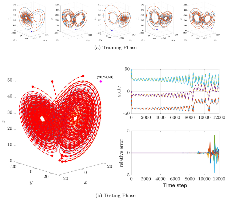
On the paper's own terms, the discovery is that a finite-dimensional linear map $\Lambda$ acting on a feature space built from $d$ delayed states and polynomial observables up to order $o$ can serve as a global iterator for nonlinear dynamics with multiple attractors, as long as the training data cover the relevant basins. The learned relation is $X = \Lambda \Upsilon$, where columns of $\Upsilon$ stack delayed states and nonlinear terms, and $\Lambda$ is found by least squares or the Moore-Penrose pseudoinverse and then iterated to predict trajectories from arbitrary initial conditions. The paper's results show that single-basin training gives an operator that only works inside that basin, whereas training with data from both sides of a basin boundary yields a single operator that generalizes across it, reproduces stable and unstable limit cycles, and tracks the Lorenz attractor for short horizons. The authors also use the iterated operator on scattered initial conditions to approximate basin boundaries, closing a feedback loop that guides further data collection.
Load-bearing premise
The user must know the correct polynomial order $o$ and a suitable feature dictionary in advance, because the paper's examples use prior knowledge of the true dynamics and the method is not shown to select this order automatically.
Editorial extensions
If this is right
- A single linear operator trained on stacked trajectories from both basins can predict test trajectories on either side of a basin boundary, where single-basin training fails.
- Iterating the learned operator from a fine grid of initial conditions approximates the basins and their boundaries without integrating the true system.
- Because the method avoids derivative estimation, it remains usable when training data carry modest Gaussian noise (about 0.1% of the signal range) without additional smoothing.
- The minimum number of training trajectories scales with the number of basins and relevant phase-space features, not with the state dimension alone.
- For a chaotic system with one global attractor, one operator trained on a few trajectories can track both lobes of the Lorenz system and extend its prediction horizon when the delay order and sampling rate are increased.
Reading between the lines
- The paper's Remark 2 means the method as presented is not yet a standalone identifier for genuinely unknown systems: automatic selection of the polynomial order $o$, or a data-driven dictionary-selection criterion, is a natural next step and the examples show performance degrades sharply when $o$ is wrong.
- The success of stacking trajectories from disjoint basins suggests that active learning could replace manual phase-space-informed sampling: train a first operator, use its approximate basin boundaries to pick new initial conditions, and retrain, following the feedback loop the paper describes qualitatively.
- The compact delayed-feature formulation could be tested as a cheap approximate-basin-boundary tool for control, where knowing which attractor a proposed input will reach matters more than an exact trajectory match.
- If the single-operator claim extends to chaotic systems, it hints that finite-dimensional linear representations of multistable dynamics may be more practically reachable than Koopman-embedding theory currently suggests.
Editorial analysis
A structured set of objections, weighed in public.
Referee Report
Summary. The paper introduces NLDM, a system identification method that combines time-delayed state augmentation (as in HODMD) with nonlinear polynomial feature lifting (as in EDMD). The unknown map Lambda is obtained by least squares from stacked trajectory data, and predictions are made by iterating Lambda on feature vectors built from the last d states. The authors propose using phase-space information, specifically attractors and their basins, to choose training trajectories; they demonstrate the method on damped oscillators, a bistable system, a double-well oscillator, a periodic-attractor system, a mixed equilibrium/limit-cycle system, and the Lorenz equations, reporting RRMSE values for training and test trajectories. The central claim is that a single linear operator, trained on trajectories from all basins, can represent nonlinear dynamics with multiple attractors and can be iterated to approximate basin boundaries.
Significance. If the claims were fully established, the method would be a practically useful extension of EDMD and HODMD, particularly for multistable systems, with a clean least-squares formulation and a sensible train/test protocol that separates initial conditions. The paper deserves credit for explicitly measuring generalization on unseen initial conditions, for testing robustness to Gaussian noise, and for making the phase-space-informed training strategy concrete through a feedback loop. However, the significance is currently limited by three gaps: no automatic selection of the polynomial order (Remark 2), no comparison with baseline methods, and only qualitative support for the basin-boundary approximation claim. The first gap is the most serious because Section 9.2 shows that a wrong order cannot be fixed by adding data.
major comments (4)
- [Section 9.2 and Remark 2] The choice of polynomial order o is load-bearing and is made using information that a data-driven identifier would not have. For Eq. (25), the paper reports that (d,o)=(2,1) and (2,2) fail, that enriching the training data does not help, and that increasing the delay order d does not help; only o=3, which matches the cubic term in the true equations, succeeds. Remark 2 states: 'for the order of the basis functions, we leveraged prior knowledge of the system dynamics used to generate the synthetic data.' No automatic model-selection criterion for o is given anywhere in the paper. Since the failure mode is not cured by more data, the general claim in the Conclusions that the algorithm 'can accurately learn the dynamics of nonlinear systems' is not established for unknown systems unless an automatic order-selection procedure is added.
- [Section 9] The paper does not include any baseline comparison. The introduction and Section 2.6 motivate NLDM as a hybrid of EDMD and HODMD and claim improved tractability and accuracy, but none of the numerical experiments in Section 9 compares NLDM against EDMD, HODMD, or SINDy on the same training and test sets. The reported RRMSE values are informative as absolute measures, but they cannot substantiate the claimed advantages over existing methods. Adding at least one baseline (e.g., EDMD and HODMD with the same feature and delay choices) is necessary to support the comparative statements.
- [Section 9.4 and Conclusions] The claim that NLDM can approximate basin boundaries is only supported by qualitative visual comparison. In Figures 6 and 7, the basins obtained by iterating the learned operator are compared visually with those produced by ODE45, and the text acknowledges differences in 'thickness and continuity'. No quantitative error measure (e.g., distance between predicted and true basin boundaries or classification accuracy of a grid of initial conditions) is reported. Moreover, the feedback loop that improves the basin-boundary approximation requires the user to inspect the learned operator and choose additional training trajectories, so the procedure does not currently constitute an automatic method. A quantitative evaluation is needed before the Conclusions' statement about approximating basin boundaries can be accepted.
- [Section 9.3, Table 2] The test RRMSE values for initial conditions near the basin boundary are orders of magnitude larger than the training RRMSE (e.g., 4.81e-2 for TS-ic [0.025,1] versus 8.53e-3 for training), and the text reports divergence for boundary initial conditions. The claim of cross-basin generalization needs a precise statement of the region of validity around the basin boundary, rather than a binary 'near vs far' discussion.
minor comments (7)
- [Eqs. (22)-(23)] The index K is already used for the number of snapshots; using it to enumerate training trajectories causes confusion. Should be Q.
- [Figure 2 caption and Section 9.2] The notation '(d, 0) = (2, 1)' should read '(d, o) = (2, 1)'.
- [Section 4, Eq. (6)] The notation '˜xk−' is undefined; write '˜x_{k-1}' or a similar explicitly defined symbol.
- [Figure 10 caption] The reference to 'Eq. (9.6)' should point to the actual system introduced in Section 9.6.
- [Title page] The MSC line reads '2000 MSC'; this should be '2020 MSC'.
- [Section 9.3] There is a typo: 'The the system of ODEs' should be 'The system of ODEs'.
- [Table 1] The entry 'NaN' for RRMSE is not explained; state whether this indicates divergence to infinity or an undefined computation.
Circularity Check
No significant circularity: test predictions are independent of the fitted operator, and the acknowledged oracle choice of polynomial order is a model-selection limitation, not a circular step.
full rationale
The paper's derivation chain is self-contained: it defines a feature map (Eq. 15), builds time-delayed nonlinear feature matrices (Eqs. 18-20), solves for the linear operator by least squares / pseudoinverse (Eq. 13 applied to Eq. 20), and then iterates that operator from test initial conditions (Section 6.1). The reported RRMSEs are computed on test trajectories whose initial conditions were not used to fit Λ (e.g., Section 9.1, TS-ic = (0,2); Section 10.1, test IC [5,1,6]), so the predictions are not fitted values by construction. The main caveat is stated explicitly in Remark 2: 'for the order of the basis functions, we leveraged prior knowledge of the system dynamics used to generate the synthetic data.' This is a genuine limitation of the data-driven identification claim, because a wrong polynomial order causes failure (Section 9.2), but it is an oracle model-selection assumption rather than a circular derivation: the paper does not define the predicted dynamics in terms of the selected order, and the test evaluations are independent of the fitting step. There is no load-bearing self-citation, no imported uniqueness theorem, and no equation in the prediction step reduces to the training target by definition. The iterative basin-refinement procedure in Section 9.4 uses the learned operator to guide additional training data, but the final comparison is against ODE45 reference solutions, so the claimed improvement is empirically checked rather than assumed. Overall, no circular step meets the standard of Eq. X = Eq. Y by construction or a fitted parameter renamed as a prediction.
Assumptions & free parameters
free parameters (5)
- Polynomial feature order o =
o=1 (Sec 9.1), o=3 (Sec 9.2-9.4), o=2 (Sec 9.5-9.6 and Sec 10)
- Time delay order d =
d=2 (Sec 9.1-9.3), d=4 (Sec 9.4), d=5 (Sec 9.6), d=3 or 4 (Sec 10)
- Number of snapshots K =
K=1000 (most examples), K=2000 (Table 1), K=4000 or 12000 (Lorenz)
- Training trajectory set (initial conditions and basin coverage) =
Varies per example: 4 ICs for oscillator, 5 ICs for Lorenz, inside/outside MFCD cylinder, both basins for…
- Gaussian noise level sigma =
0.1% of signal range in most examples
assumptions (4)
- domain assumption The learned finite-dimensional linear map on the feature space approximates the true nonlinear dynamics well enough to be iterated over long prediction horizons.
- ad hoc to paper Polynomial features of order o can represent the vector field or its Koopman closure.
- domain assumption A finite set of trajectories, one per basin, provides sufficient sampling for a least-squares operator that generalizes inside those basins.
- domain assumption Iterating the learned operator on a grid of initial conditions yields a valid approximation of the true basin boundaries.
Cite this review
Pith. "Pith review of Data-Driven Model Identification Using Time Delayed Nonlinear Maps for Systems with Multiple Attractors." pith.science (2026). https://pith.science/paper/W7IT7UWB
@misc{pith2026241110910,
  author       = {Pith},
  title        = {Pith review of: Data-Driven Model Identification Using Time Delayed Nonlinear Maps for Systems with Multiple Attractors},
  year         = {2026},
  howpublished = {\url{https://pith.science/paper/W7IT7UWB}},
  note         = {Machine review of arXiv:2411.10910}
}
read the original abstract
This study presents a method, along with its algorithmic and computational framework implementation, and performance verification for dynamical system identification. The approach incorporates insights from phase space structures, such as attractors and their basins. By understanding these structures, we have improved training and testing strategies for operator learning and system identification. Our method uses time delay and non-linear maps rather than embeddings, enabling the assessment of algorithmic accuracy and expressibility, particularly in systems exhibiting multiple attractors. This method, along with its associated algorithm and computational framework, offers broad applicability across various scientific and engineering domains, providing a useful tool for data-driven characterization of systems with complex nonlinear system dynamics.
Figures


Figures from the paper (9 more)


Reference graph
Works this paper leans on
-
[1]
P. J. Schmid, Dynamic mode decomposition and its variants, Annual Review of Fluid Mechanics 54 (1) (2022) 225–254
2022
-
[2]
S. L. Brunton, M. Budišić, E. Kaiser, J. N. Kutz, Modern Koopman theory for dynamical systems, SIAM Rev. 64 (2021) 229–340. URL https://api.semanticscholar.org/CorpusID:232035467
work page 2021
-
[3]
L. Lu, P. Jin, G. Pang, Z. Zhang, G. E. Karniadakis, Learning nonlinear operators via deeponet based on the universal approximation theorem of operators, Nature Machine Intelligence 3 (3) (2021) 218–229.doi: 10.1038/s42256-021-00302-5. URL http://dx.doi.org/10.1038/s42256-021-00302-5
-
[4]
Raissi, P
M. Raissi, P. Perdikaris, G. E. Karniadakis, Physics-informed neural networks: A deep learning framework for solving forward and inverse problems involving nonlinear partial differential equations, Journal of Computational Physics 378 (2019) 686–707
2019
-
[5]
P. J. Schmid, Dynamic mode decomposition of numerical and experi- mental data, Journal of fluid mechanics 656 (2010) 5–28
2010
-
[6]
F. Lusseyran, F. Guéniat, J. Basley, C. Douay, L. Pastur, T. Faure, P. J. Schmid, Flow coherent structures and frequency signature: Application of the dynamic modes decomposition to open cavity flow, in: Journal of Physics: Conference Series, Vol. 318, IOP Publishing, 2011, p. 042036
work page 2011
- [7]
-
[8]
P. J. Schmid, L. Li, M. P. Juniper, O. Pust, Applications of the dynamic mode decomposition, Theoretical and computational fluid dynamics 25 (2011) 249–259
work page 2011
Show all 26 references
-
[9]
B. O. Koopman, Hamiltonian systems and transformation in Hilbert space, Proceedings of the National Academy of Sciences 17 (5) (1931) 315–318
1931
-
[10]
Mauroy, I
A. Mauroy, I. Mezić, A spectral operator-theoretic framework for global stability, in: 52nd IEEE Conference on Decision and Control, IEEE, 2013, pp. 5234–5239
2013
-
[11]
M. O. Williams, I. G. Kevrekidis, C. W. Rowley, A data–driven ap- proximation of the Koopman operator: Extending dynamic mode de- composition, Journal of Nonlinear Science 25 (6) (2015) 1307–1346. doi:10.1007/s00332-015-9258-5. URL https://doi.org/10.1007/s00332-015-9258-5
2015 doi
-
[12]
S. L. Brunton, B. W. Brunton, J. L. Proctor, J. N. Kutz, Koopman invariant subspaces and finite linear representations of nonlinear dy- namical systems for control, PloS one 11 (2) (2016) e0150171
2016
-
[13]
J. Page, R. R. Kerswell, Koopman mode expansions between simple invariant solutions, Journal of Fluid Mechanics 879 (2019) 1–27
2019
-
[14]
Bakker, K
C. Bakker, K. E. Nowak, W. S. Rosenthal, Learning Koopman operators for systems with isolated critical points, in: 2019 IEEE 58th Conference on Decision and Control (CDC), IEEE, 2019, pp. 7733–7739
2019
-
[15]
Bakker, T
C. Bakker, T. Ramachandran, W. S. Rosenthal, Learning bounded Koopman observables: Results on stability, continuity, and controlla- bility, arXiv preprint arXiv:2004.14921 (2020)
2020 arXiv
-
[16]
M. D. Kvalheim, S. Revzen, Existence and uniqueness of global Koop- man eigenfunctions for stable fixed points and periodic orbits, Physica D: Nonlinear Phenomena 425 (2021) 132959
2021
-
[17]
Arathoon, M
P. Arathoon, M. D. Kvalheim, Koopman embedding and super- linearization counterexamples with isolated equilibria, arXiv preprint arXiv:2306.15126 (2023)
2023 arXiv
-
[18]
Z. Liu, N. Ozay, E. D. Sontag, Properties of immersions for systems with multiple limit sets with implications to learning Koopman embeddings, arXiv preprint arXiv:2312.17045 (2023). 39
2023 arXiv
-
[19]
Breunung, F
T. Breunung, F. Kogelbauer, Learning global linear representations of truly nonlinear dynamics, arXiv preprint arXiv:2408.03437 (2024)
2024 arXiv
-
[20]
Le Clainche, J
S. Le Clainche, J. M. Vega, Higher order dynamic mode decomposition, SIAM Journal on Applied Dynamical Systems 16 (2) (2017) 882–925
2017
-
[21]
S. L. Brunton, J. L. Proctor, J. N. Kutz, Discovering governing equa- tions from data by sparse identification of nonlinear dynamical systems, Proceedings of the national academy of sciences 113 (15) (2016) 3932– 3937
2016
-
[22]
Cortiella, K.-C
A. Cortiella, K.-C. Park, A. Doostan, Sparse identification of non- linear dynamical systems via reweighted ℓ1-regularized least squares, Computer Methods in Applied Mechanics and Engineering 376 (2021) 113620
2021
-
[23]
Takens, Detecting strange attractors in turbulence, in: Dynamical Systems and Turbulence, Warwick 1980, Springer, 1981, pp
F. Takens, Detecting strange attractors in turbulence, in: Dynamical Systems and Turbulence, Warwick 1980, Springer, 1981, pp. 366–381
1980
-
[24]
J. C. Robinson, Takens’ embedding theorem for infinite-dimensional dynamical systems, Nonlinearity 12 (1999) 1263–1275
1999
-
[25]
Groun, M
N. Groun, M. Villalba-Orero, E. Lara-Pezzi, E. Valero, J. Garicano- Mena, S.LeClainche, Higherorderdynamicmodedecomposition: From fluid dynamics to heart disease analysis, Computers in Biology and Medicine 144 (2022) 105384
2022
-
[26]
Sparrow, The Lorenz equations: bifurcations, chaos, and strange attractors, Vol
C. Sparrow, The Lorenz equations: bifurcations, chaos, and strange attractors, Vol. 41, Springer Science & Business Media, 2012. 40
2012
Reviewed August 12, 2026 · model on record in the stance chip above.
Discussion (0). Continue with ORCID to comment.