REVIEW 3 major objections 6 minor 43 references
Testing the generalized conjugate field formalism in the kinetic Ising model with nonantisymmetric magnetic fields: A Monte Carlo simulation study
T0 review · 3 major / 6 minor · reviewed 2026-08-12 · deepseek-v4-flash
Pith's one-line read In a honeycomb-lattice kinetic Ising model, the generalized conjugate field formalism survives a second harmonic field, but the critical exponent δ drops from ~15 to ~12.88.
desk verdict A clean but incremental check of the H* formalism on a honeycomb lattice; the exponent-deviation claim is off-critical and should be withdrawn or re-derived. read the letter →
The pith
A machine-rendered reading of the paper's core claim, the machinery that carries it, and where it could break.
The reading
What carries the argument
The central object is the generalized conjugate field $H^{*}$, defined for the field sequence $H(t) = H_b + H_0 \sin(2\pi t/P) + H_2 \sin(4\pi t/P)$ as $H^{*} = H_b + \Delta H$, where $\Delta H = -[H_b(Q) + H_b(-Q)]/2$. This construction is designed to restore the odd symmetry $Q(H^{*}) = -Q(-H^{*})$, which the bias field $H_b$ alone fails to provide once the second harmonic $H_2$ breaks the half-wave anti-symmetry. The paper's evidence is built on Monte Carlo simulations with Metropolis dynamics, Binder cumulant crossings to locate the critical half-period $t_{1/2}^{c} = 57$, and log-log fits of $\langle Q \rangle$ versus $H^{*}$ to extract the exponent $\delta_d$.
What would settle it
Find the transition point for $H_2/J = 0.01$ by locating the crossing of Binder cumulant curves for different lattice sizes; if that crossing is not at $t_{1/2}^c = 57$, repeat the exponent fit at the shifted point and check whether the exponent returns to about $15$.
Extended reading notes
Core claim
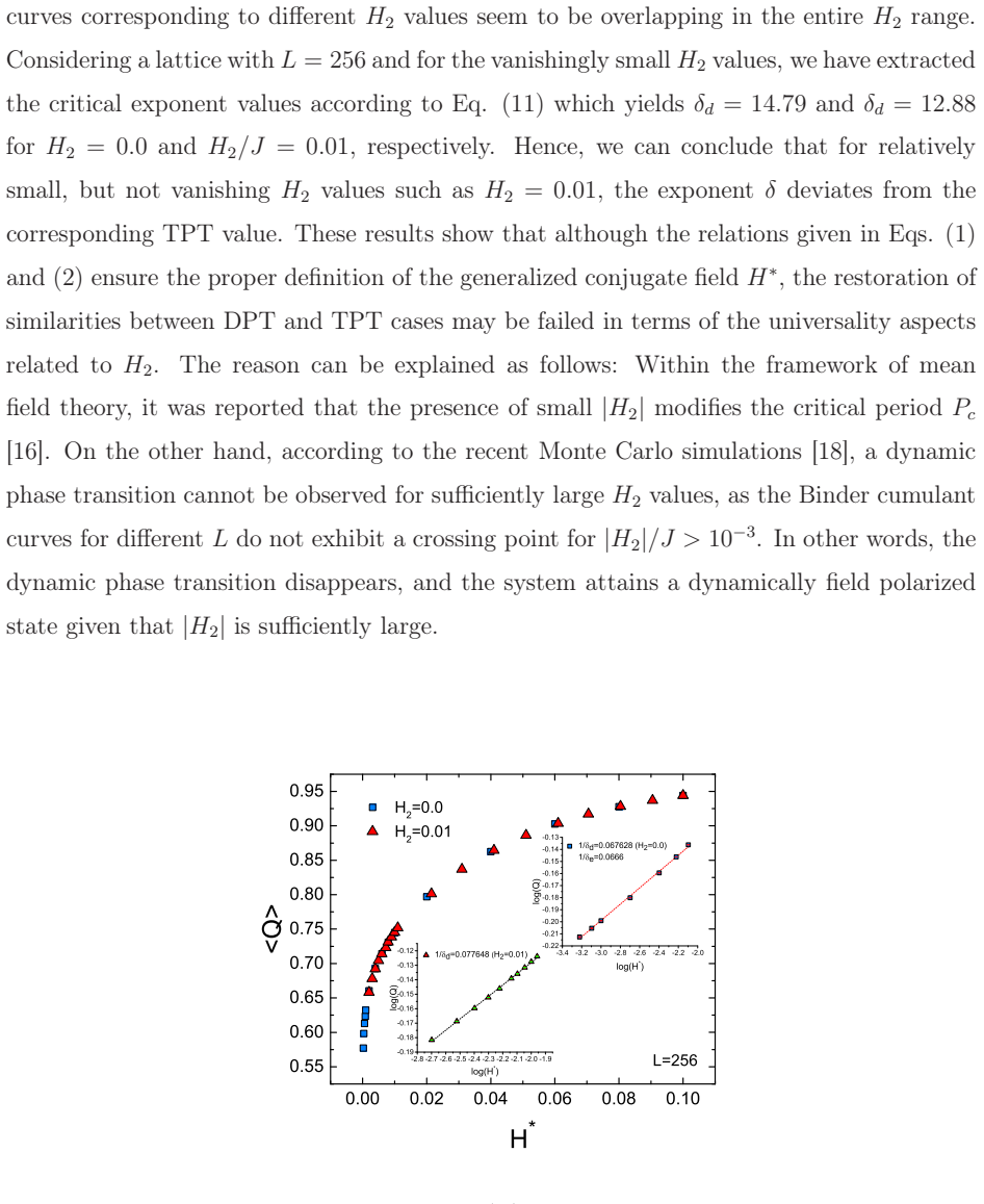
The paper reports that the generalized conjugate field $H^{*} = H_b + \Delta H$, with $\Delta H = -[H_b(Q) + H_b(-Q)]/2$, remains the correct conjugate field for the dynamic order parameter $Q$ in a kinetic Ising model on a honeycomb lattice even when a second magnetic field component of amplitude $H_2$ and period $P/2$ breaks the half-wave anti-symmetry of the driving field. For nonzero $H_2$, plots of $\langle Q \rangle$ versus $H^{*}$ are antisymmetric about zero and curves for different $|H_2|$ collapse onto one another, verifying the formalism. At the same time, the dynamic critical exponent $\delta_d$ obtained from the scaling $\langle Q \rangle \propto (H^{*})^{1/\delta}$ at the critical period deviates from the equilibrium 2D Ising value: $\delta_d \approx 14.79$ for $H_2 = 0$ and $\delta_d \approx 12.88$ for $H_2/J = 0.01$, compared with $\delta_e = 15$. The author also finds that for sufficiently large $|H_2|$ the dynamic phase transition disappears and the system enters a dynamically field-polarized state.
Load-bearing premise
The paper's central assumption is that turning on the small second-field component $H_2/J = 0.01$ does not move the transition point from its zero-field value $t_{1/2}^c = 57$; if the transition point shifts, the extracted exponent $12.88$ is an off-critical number, not a true critical exponent.
Editorial extensions
If this is right
- For half-wave antisymmetric field sequences ($H_2 = 0$, $H_b = 0$), the honeycomb-lattice kinetic Ising model shows a second-order dynamic phase transition at $t_{1/2}^{c} = 57$, and the bias field $H_b$ acts as the conjugate field of $Q$.
- When a second harmonic component $H_2$ is present, $H_b$ is no longer the conjugate field; the generalized field $H^{*}$ defined by Eqs. (1)-(2) restores $Q(H^{*}) = -Q(-H^{*})$ and collapses $\langle Q \rangle$ versus $H^{*}$ curves for different $|H_2|$.
- The dynamic critical exponent $\delta_d$ at $H_2/J = 0.01$ is about $12.88$ instead of the equilibrium 2D Ising value $15$, indicating that universality between dynamic and equilibrium criticality is not preserved in this generalized-field setting.
- For sufficiently large $|H_2|$, the dynamic phase transition is destroyed and the system becomes dynamically field polarized, consistent with the absence of a Binder cumulant crossing for $|H_2|/J > 10^{-3}$.
- The author notes that extending the conclusions to three-dimensional lattices is straightforward.
Reading between the lines
- Because the paper does not perform a Binder cumulant crossing for $H_2/J = 0.01$, the value $\delta_d \approx 12.88$ may be an effective off-critical exponent; a rerun at the true, possibly shifted, critical period could bring $\delta$ closer to $15$ and would test whether the universality breakdown is real.
- The simultaneous collapse of $\langle Q \rangle$ versus $H^{*}$ and the drift of $\delta$ raise the possibility that $H^{*}$ is the correct scaling variable but corrections to scaling grow with $H_2$; an analysis with a field-dependent effective exponent could reconcile the two observations.
- The honeycomb lattice's low coordination number could amplify the exponent shift relative to denser lattices; comparing $\delta_d(H_2)$ on square, kagome, and honeycomb lattices would show whether the deviation is a universal feature of broken half-wave anti-symmetry.
- The dynamically field-polarized state for large $H_2$ is a concrete prediction that could be tested experimentally by driving a thin-film ferromagnet with a two-harmonic field sequence and measuring the time-averaged magnetization as a function of $H_2$.
Editorial analysis
A structured set of objections, weighed in public.
Referee Report
Summary. The manuscript reports Monte Carlo simulations of the kinetic Ising model on a honeycomb lattice driven by a time-dependent magnetic field with a fundamental component H0 and a second harmonic H2 of period P/2. For H2=0, the authors locate a dynamic phase transition at half-period t1/2^c=57 via Binder cumulant crossings and finite-size scaling of the variance, and they confirm that the bias field Hb acts as the conjugate field. For non-zero H2, they compute the generalized conjugate field H* of Quintana and Berger from Eqs. (1)-(2) and find that Q(H*) is antisymmetric and that curves for different |H2| collapse (Fig. 4d). They then extract a dynamic critical exponent delta_d from fits of Q(H*) near H*=0 at the fixed half-period t1/2=57, reporting delta_d=14.79 for H2=0 and delta_d=12.88 for H2/J=0.01, and interpret the latter as a significant deviation from the equilibrium 2D Ising value delta_e=15.
Significance. If the central claims hold, the paper would extend the generalized conjugate field formalism to a new lattice geometry (honeycomb) and demonstrate a breakdown of universality in the dynamic critical exponents for small but non-vanishing H2. The data collapse in Fig. 4d is a non-trivial qualitative confirmation of the formalism and is the strongest part of the manuscript. However, the claim of an exponent change is not adequately supported: the H2=0.01 exponent is extracted at a critical period calibrated only for H2=0, and the manuscript itself cites a recent study (Ref. [18]) finding no dynamic phase transition for |H2|/J > 1e-3. The reported exponent values also lack error bars. The qualitative confirmation of the formalism is valuable, but the quantitative exponent claim needs substantial additional analysis before it can be accepted.
major comments (3)
- [Sec. III, Fig. 5 and Eq. (11)] The critical half-period t1/2^c=57 is determined exclusively for H2=0 in Fig. 3 via Binder cumulant crossings and chi_Q scaling. For H2/J=0.01, no Binder crossings, chi_Q peaks, or any finite-size analysis are reported. Since Eq. (11) is only valid at P=Pc, and the paper acknowledges in the same section that mean-field theory predicts a shift in Pc with H2 (Ref. [16]) and that Ref. [18] finds no dynamic phase transition for |H2|/J > 1e-3, the H2=0.01 curve at t1/2=57 is not justified as a critical isotherm. The resulting delta_d=12.88 is therefore an effective off-critical slope, not evidence that the generalized conjugate field formalism changes the dynamic critical exponent.
- [Sec. III, Fig. 5] The values delta_d=14.79 and delta_d=12.88 are quoted without statistical uncertainties. The log-log insets in Fig. 5 do not show error bars or the range over which the power law was fitted. Given that the jackknife errors are stated to be smaller than the data points elsewhere, the paper should report error bars on these slopes and on the fit range; otherwise the claimed deviation from delta_e=15 cannot be assessed.
- [Sec. III, paragraph after Fig. 5] The manuscript states that for |H2|/J > 1e-3 the dynamic phase transition disappears and the system becomes dynamically field polarized, citing Ref. [18]. This statement is directly contradictory to the use of H2/J=0.01 in a critical scaling relation, and the contradiction is not resolved in the text. The authors should either demonstrate that the transition still exists at H2/J=0.01 on the honeycomb lattice by locating the new critical period, or explicitly limit their exponent claim to fields below the polarized threshold. If the latter, the claim that a small H2 changes the exponent would be unsupported.
minor comments (6)
- [Abstract and Ref. [16]] The reference to Quintana and Berger is missing the year: it reads "Phys. Rev. E 104, 044125 (202)" and should be "(2021)".
- [Title page] The first word of the title is typeset as "T esting" with an unwanted space; this should be corrected.
- [Sec. II, paragraph 1] "We empose periodic boundary conditions" should be "We impose periodic boundary conditions".
- [Sec. III, Fig. 2d discussion] "This can bee seen" should be "This can be seen".
- [References] References [23] and [35] are the same paper (Y. Yüksel, Phys. Rev. E 108, 034125 (2023)); they should be merged or renumbered.
- [Sec. III, Eq. (11) paragraph] The phrase "the following scaling relation can be verified or not" is awkward; it should be rephrased, e.g., "we now test whether the following scaling relation holds".
Circularity Check
Antisymmetry of Q(H*) is built into the H* definition via Eq. (2); collapse and exponent remain independent, though the H2=0.01 exponent uses an H2=0 critical period.
-
self definitional
[Sec. III, paragraph following Fig. 4(d); Eqs. (1) and (2)]
"When ⟨Q⟩ is plotted as a function of H ∗ which is calculated with the help of Eqs. (1) and (2), we see that the half-wave anti-symmetry property is restored and ⟨Q⟩ vs H ∗ curves corresponding to different |H2| values collapse onto each other."
H* is constructed from the measured Q(Hb) curve via Eq. (2), ΔH = −1/2[Hb(Q)+Hb(−Q)]. Writing Hb = h(Q), the construction gives H*(Q) = (1/2)[h(Q)−h(−Q)], which is an odd function of Q for any single-valued measured h. Hence Q plotted against H* obeys Q(H*) = −Q(−H*) identically. The statement that the half-wave anti-symmetry property is 'restored' after computing H* from Eqs. (1)–(2) is therefore a consequence of the definition, not an empirical test. The non-circular content lies in the separate claims: collapse of curves for different |H2| and the extracted δd value, neither of which is forced by the antisymmetrizing construction.
full rationale
The only genuinely circular step is the 'restored half-wave anti-symmetry' in Q(H*). Since Eq. (2) defines ΔH by antisymmetrizing the measured inverse function Hb(Q), the resulting H*(Q) is odd by construction, so Q(H*) is odd regardless of the underlying physics. Thus the statement that the anti-symmetry is restored after applying Eqs. (1)–(2) is a restatement of the definition, not a test. The nontrivial content lies elsewhere: the collapse of Q(H*) curves for different |H2| onto one master curve is not implied by the definition, and the extracted δd is a fitted slope rather than a built-in consequence of H*. The δd = 12.88 result is, however, weakened by an off-critical extrapolation: t_{1/2}^c = 57 was located by Binder crossings and χ_Q scaling only for H2 = 0 (Fig. 3), while the paper itself cites Ref. [18] as finding no dynamic phase transition for |H2|/J > 10^-3 and acknowledges the mean-field result that small H2 modifies Pc. Applying Eq. (11), which is valid only at P = Pc, at H2/J = 0.01 therefore measures an off-critical effective slope in a regime where the cited literature says the transition disappears. This is a correctness and validity risk, not a circularity, so it does not raise the circularity score beyond the partial self-definitional issue. The self-citations and the Quintana-Berger formalism are not load-bearing in a circular way: the H2 = 0 check from Ref. [23] is an independent numerical comparison, and the formalism is explicitly imported from prior work rather than derived inside this paper. Overall the derivation has independent content in the collapse and exponent claims, but the central antisymmetry verification is partly definitional, giving a partial circularity score of 4.
Assumptions & free parameters
free parameters (5)
- H0/J =
0.3
- T/Tc =
0.8
- H2/J =
0.01 (and ±0.01, ±0.02, ±0.03)
- t_{1/2}^c (half-period) =
57
- δd (dynamic critical exponent) =
14.79 (H2=0), 12.88 (H2=0.01)
assumptions (4)
- domain assumption Equilibrium transition temperature Tc/J = 1.519 for the honeycomb Ising model
- domain assumption The generalized conjugate field definition H* = Hb + ΔH, with ΔH = -1/2[Hb(Q)+Hb(-Q)] from Refs. [16,17], is the correct construction for non-antisymmetric fields
- domain assumption Q(H* → 0) ∝ (H*)^{1/δ} holds at P = Pc even for H2 ≠ 0
- ad hoc to paper The critical half-period determined at H2=0 remains valid for H2/J=0.01
Cite this review
Pith. "Pith review of Testing the generalized conjugate field formalism in the kinetic Ising model with nonantisymmetric magnetic fields: A Monte Carlo simulation study." pith.science (2026). https://pith.science/paper/LBR3QBT2
@misc{pith2026241113119,
  author       = {Pith},
  title        = {Pith review of: Testing the generalized conjugate field formalism in the kinetic Ising model with nonantisymmetric magnetic fields: A Monte Carlo simulation study},
  year         = {2026},
  howpublished = {\url{https://pith.science/paper/LBR3QBT2}},
  note         = {Machine review of arXiv:2411.13119}
}
abstract
We have performed Monte Carlo simulations for the investigation of dynamic phase transitions on a honeycomb lattice which has garnered a significant amount of interest from the viewpoint of tailoring the intrinsic magnetism in two-dimensional materials. For the system under the influence of time-dependent magnetic field sequences exhibiting the half-wave anti-symmetry, we have located a second order dynamic phase transition between dynamic ferromagnetic and dynamic paramagnetic states. Particular emphasis was devoted for the examination of the generalized conjugate field formalism previously introduced in the kinetic Ising model [\color{blue}Quintana and Berger, Phys. Rev. E \textbf{104}, 044125 (202); Phys. Rev. E \textbf{109}, 054112] \color{black}. Based on the simulation data, in the presence of a second magnetic field component with amplitude $H_{2}$ and period $P/2$, the half-wave anti-symmetry is broken and the generalized conjugate field formalism is found to be valid for the present system. However, dynamic scaling exponent significantly deviates from its equilibrium value along with the manifestation of a dynamically field polarized state for non-vanishing $H_{2}$ values.
Figures


Figures from the paper (2 more)

Reference graph
Works this paper leans on
- [16]
-
[18]
Z. D. Vatansever, E. Vatansever, A. Berger, A. Vasilopou los, and N. G. Fytas, arXiv:2409.20152 (2024), 10.48550/arXiv.2409.20152
work page Pith review arXiv doi:10.48550/arxiv.2409.20152 2024
- [1]
-
[2]
W. S. Lo and R. A. Pelcovits, Phys. Rev. A 42, 7471 (1990)
1990
- [3]
- [4]
-
[5]
D. T. Robb, Y. H. Xu, O. Hellwig, J. McCord, A. Berger, M. A. N ovotny, and P. A. Rikvold, Phys. Rev. B 78, 134422 (2008)
work page 2008
-
[6]
B. K. Chakrabarti and M. Acharyya, Rev. Mod. Phys. 71, 847 (1999)
work page 1999
Show all 43 references
-
[7]
Riego, P
P. Riego, P. Vavassori, and A. Berger, Physica B 549, 13 (2018)
2018
-
[8]
Korniss, W
G. Korniss, W. C. J., P. A. Rikvold, and M. A. Novotny, Phys . Rev. E 63, 016120 (2000)
2000
-
[9]
G. M. Buendía and P. A. Rikvold, Phys. Rev. E 78, 051108 (2008)
2008
-
[10]
G. M. Buendía and P. A. Rikvold, Phys. Rev. B 96, 134306 (2017)
2017
-
[11]
Mendes, G
C. Mendes, G. M. Buendia, and P. A. Rikvold, Phys. Rev. E 110, 044133 (2024)
2024
-
[12]
Riego, P
P. Riego, P. Vavassori, and A. Berger, Phys. Rev. Lett. 118, 117202 (2017)
2017
-
[13]
J. M. M. Ramírez, E. Oblak, G. Riego, P. Campillo, J. Osor io, and A. Arnache, O. and. Berger, Phys. Rev. E 102, 022804 (2020)
2020
-
[14]
Berger, J
A. Berger, J. F. Mitchell, D. J. Miller, and S. D. Bader, J. A ppl. Phys. 89, 6851 (2001)
2001
-
[15]
McKenzie, M
S. McKenzie, M. F. Sykes, and D. S. Gaunt, J. Phys. A: Math . Gen. 12, 743 (1979)
1979
-
[17]
Quintana and A
M. Quintana and A. Berger, Phys. Rev. E 109, 054112 (2024)
2024
-
[19]
K. S. Novoselov, A. K. Geim, S. V. Morozov, D. Jiang, Y. Zh ang, S. V. Dubonos, I. V. Grigorieva, and A. A. Firsov, Science 306, 666 (2004)
2004
-
[20]
2K (RuCl3) [26]
and Tc = 14 . 2K (RuCl3) [26]. According to the crystal structure analysis of these materials, magnetic atoms are arranged in a honeycomb latti ce formation. From the perspectives of DPT and 2D magnetism, our aim is to ex amine the recent developments such as applicability of ...
-
[21]
Huang, J
C. Huang, J. Zhou, H. Wu, K. Deng, P. Jena, and E. Kan, Phys . Rev. B 95, 045113 (2017)
2017
-
[22]
Huang, G
B. Huang, G. Clark, E. Navarro-Moratalla, D. R. Klein, R. Cheng, K. L. Seyler, D. Zhong, E. Schmidgall, M. A. McGuire, D. H. Cobden, W. Yao, D. Xiao, P. Jarillo-Herrero, and X. Xu, Nature 546, 270 (2017)
2017
-
[23]
Yüksel, Phys
Y. Yüksel, Phys. Rev. E 108, 034125 (2023). 13
2023
-
[24]
Vatansever, Physica A 511, 232 (2018)
E. Vatansever, Physica A 511, 232 (2018)
2018
-
[25]
Y. Xue, Z. Shen, and Z. Wu, J. Appl. Phys. 132, 053901 (2022)
2022
-
[26]
Webster and J
L. Webster and J. A. Yan, Phys. Rev. B 98, 144411 (2018)
2018
-
[27]
M. E. J. Newman and G. Barkema, Monte Carlo Methods in Statistical Physics (Oxford Uni- versity Press, 2001)
2001
-
[28]
Sarikurt, Y
S. Sarikurt, Y. Kadioglu, F. Ersan, E. Vatansever, O. U. Aktürk, Y. Yüksel, U. Akinci, and E. Aktürk, Phys. Chem. Chem. Phys. 20, 997 (2018)
2018
-
[29]
S. W. Sides, P. A. Rikvold, and M. A. Novoty, Phys. Rev. Le tt. 81, 834 (1998)
1998
-
[30]
Binder and D
K. Binder and D. Landau, A Guide to Monte Carlo Simulations in Statistical Physics (Cam- bridge University Press, 2009)
2009
-
[31]
M. E. Fisher, Rep. Prog. Phys. 30, 615 (1967)
1967
-
[32]
P. A. Rikvold, H. Tomita, S. Miyashita, and S. W. Sides, P hys. Rev. E 49, 5080 (1994)
1994
-
[33]
Binder, Z
K. Binder, Z. Phys. B: Condens. Matter 43, 119 (1981)
1981
-
[34]
M. E. Fisher, Critical Phenomena, edited by M. S. Green (Academic Press, London UK, 1971)
1971
-
[35]
Yüksel, Phys
Y. Yüksel, Phys. Rev. E 108, 034125 (2023)
2023
-
[36]
Park and M
H. Park and M. Pleimling, Phys. Rev. E 87, 032145 (2013)
2013
-
[37]
D. T. Robb, P. A. Rikvold, A. Berger, and M. A. Novoty, Phys . Rev. E 76, 021124 (2007)
2007
-
[38]
Z. D. Vatansever, Phys. Rev. E 106, 054143 (2023)
2023
-
[39]
Kamieniarz and H
G. Kamieniarz and H. W. J. Blöte, J. Phys. A: Math. Gen. 26, 201 (1993)
1993
-
[40]
S. W. Sides, P. A. Rikvold, and M. A. Novoty, Phys. Rev. E 59, 2710 (1999)
1999
-
[41]
Salas and A
J. Salas and A. D. Sokal, J. Stat. Phys. 98, 551 (2000). 14
2000
-
[42]
Selke and L
W. Selke and L. N. Shchur, J. Phys. A: Math. Gen. 38, L739 (2005)
2005
-
[256]
1 × 10⁴ period cycles of the oscillating field were considered and the initial 103 cycles were discarded for thermalization
In order to calculate the physical quantities, 1. 1 × 10⁴ period cycles of the oscillating field were considered and the initial 103 cycles were discarded for thermalization. Hence, the computational time need for measuring the quantities de pends on the period P . In the absen...
Reviewed August 12, 2026 · model on record in the stance chip above.
Discussion (0). Continue with ORCID to comment.