REVIEW 4 major objections 6 minor 27 references
Robust Convergency Indicator using MIMO-PI Controller in the presence of disturbances
T0 review · 4 major / 6 minor · reviewed 2026-08-12 · deepseek-v4-flash
Pith's one-line read A computable robustness indicator predicts when MIMO-PI controllers force errors into an exponentially shrinking ball, even with bounded disturbances.
desk verdict The core theorem overreaches: local Hurwitz stability of A_K(0) does not imply global exponential convergence, and the counterexample is valid—still, the R_K/I_K tuning machinery is a novel and potentially useful heuristic. read the letter →
The pith
A machine-rendered reading of the paper's core claim, the machinery that carries it, and where it could break.
The reading
What carries the argument
The load-bearing object is the augmented matrix $A_K(0)$ from the velocity-form linearization: $A_K(0) = \begin{pmatrix} \frac{\partial f}{\partial x}(0) + \frac{\partial f}{\partial u}(0) K_P & \frac{\partial f}{\partial u}(0) K_I \\ I_n & 0 \end{pmatrix}$. This matrix captures the effect of both proportional and integral gains on the coupled dynamics of $(\dot x, x)$. The argument rests on showing that if this matrix is Hurwitz and the plant is $\beta_f$-smooth with $\|\dot d\| \le L_d$, then the Lyapunov function $V(s) = f_s(s)^T P f_s(s)$ yields a dissipation inequality that bounds the trajectory in terms of $R_K$ and $I_K$.
What would settle it
Run a nonlinear simulation of the closed-loop system with a fixed Hurwitz $A_K(0)$, a nonzero initial condition far from the origin, and a bounded random perturbation $\dot d$ with $\|\dot d\| \le L_d$. If the error norm $\|s(t)\|_2$ either exceeds the predicted radius $2 L_d L_f I_K$ after a long time or decays slower than the predicted exponential rate $R_K$ (e.g., by fitting an exponential envelope to $\|s(t)\|$), the theorem's global claim is false. To be conclusive, test initial conditions at several distances and disturbance amplitudes $L_d$; the theory says convergence to the ball must occur from any initial state, so a single counterexample trajectory suffices.
Extended reading notes
Core claim
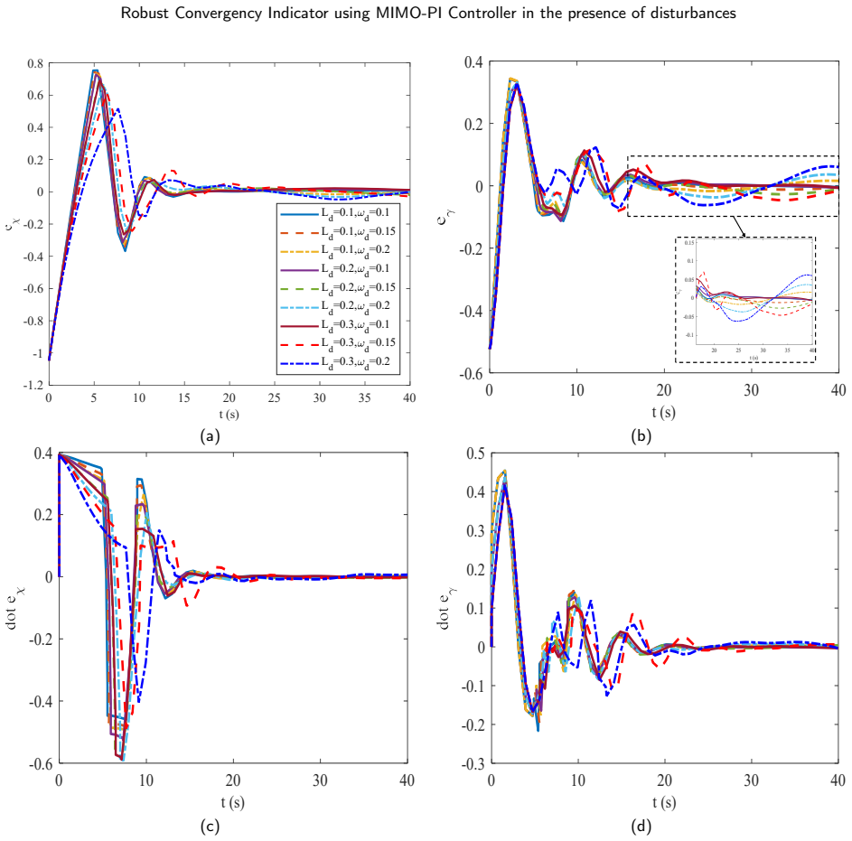
The central discovery is that the robustness of a MIMO-PI controller for a perturbed nonlinear system can be quantified by two scalar indicators extracted from the origin of the velocity-form augmented system. Specifically, for $\dot x = f(x,u) + d$ with $\|\dot d\| \le L_d$, the controller $u = K_P x + K_I \int_0^t x\,dt$ leads to the augmented dynamics $\dot s = A_K(s)s + d_s$ where $s = (\dot x, x)$ and $A_K(0)$ is the Jacobian of the velocity form at the origin. The paper's Theorem 2 states that if $\mathrm{Re}[A_K(0)] < 0$, then there exists a positive-definite $P$ and $\varepsilon(0)>0$ such that the state converges exponentially to the ball $B(0, 2 L_d L_f I_K)$ with rate $R_K = \varepsilon(0)/\lambda_{\max}(P)$ and $I_K = \|A_K(0)^{-1}\|_2 \lambda_{\max}^2(P)/(\varepsilon(0)\lambda_{\min}(P))$. These indicators are then computed by solving a convex eigenvalue problem (EVP) for the scaled Lyapunov matrix $Q_K$, and the gains are optimized by maximizing $R_K$ subject to $I_K \le I^*$ and input constraints. The paper validates the theory on a Duffing oscillator and on a fixed-wing aircraft kinematic model under sinusoidal disturbances, showing that larger $R_K$ correlates with lower ITAE, overshoot, and post-stabilization variance.
Load-bearing premise
The main load-bearing premise is that the stability of the linearized augmented matrix $A_K(0)$ at the origin guarantees the claimed exponential convergence of the nonlinear closed-loop system for all initial conditions, even though the Lyapunov inequality is only verified at the single point $\Omega = \{0\}$.
Editorial extensions
If this is right
- If $R_K$ and $I_K$ are valid predictors, gain tuning for MIMO-PI controllers on disturbed nonlinear plants becomes a convex optimization problem in $Q_K$ plus a scalar search, rather than a black-box heuristic search.
- The paper's Theorem 2 implies that any gains making $A_K(0)$ Hurwitz guarantee exponential convergence to a bounded region, so robustness can be certified without simulating the full nonlinear closed-loop system.
- The optimization model in Eq. (54) shows that the maximal convergence rate can be pursued while enforcing actuator limits at the initial instant, which is directly applicable to flight control and similar input-constrained problems.
- The indicators $R_K$ and $I_K$ provide a quantitative trade-off: larger rate $R_K$ does not automatically yield a smaller ultimate ball $I_K$; the relationship involves the condition number of $Q_K$, so tuning should consider both metrics.
- The Duffing and aircraft experiments suggest that the indicators can rank controller gains by transient and steady-state error in a prescriptive way, making them usable as surrogate objectives in auto-tuning tools.
Reading between the lines
- A natural testable extension is to check whether the same $R_K$/$I_K$ framework applies when the disturbance bound is on $\|d\|$ rather than $\|\dot d\|$; Theorem 1 uses $L_d$ for $d$, while Theorem 2 requires $\|\dot d\| \le L_d$, which may be overly restrictive for constant or step disturbances.
- Because the proof only verifies the Lyapunov inequality at the origin, a more careful region-of-attraction analysis would be needed to guarantee that trajectories starting far away actually stay within the region where $A_K(s)$ remains stable; without that, the 'global' statement is only local in practice.
- The indicator $I_K$ depends on $\|A_K(0)^{-1}\|_2$, so the ball radius grows when $A_K(0)$ is nearly singular. This suggests a design trade-off that the paper does not fully exploit: explicitly shaping the eigenvalues of $A_K(0)$ (e.g., via LMI-based pole placement) could directly reduce $I_K$ for a fixed $R_K$.
- The experiments vary $K$ by a single scalar perturbation $\varepsilon$; a more comprehensive validation would sample the gain space randomly around $K^*$ and test whether $R_K$ and $I_K$ remain monotone predictors of the performance metrics, which is exactly what the indicators claim to do.
Editorial analysis
A structured set of objections, weighed in public.
Referee Report
Summary. The paper proposes a quantitative robustness indicator for MIMO-PI controllers applied to general perturbed nonlinear systems. It first states a Lyapunov-based theorem (Theorem 1) on exponential convergence of trajectories to a 'global random attractor', then derives a velocity-form augmented system for the closed loop with a MIMO-PI controller and defines two indicators: R_K, the exponential convergence rate, and I_K, the radius of the ultimate attractor. The indicators are computed through an eigenvalue problem (EVP), and an optimization model is proposed to tune the controller gains subject to input-magnitude and input-rate constraints. The claims are supported by simulations on a Duffing oscillator and on a fixed-wing kinematic model, comparing controllers with different R_K and I_K values.
Significance. If the global exponential-convergence claim were correct, the paper would offer a practical, optimization-ready tuning metric for MIMO-PI controllers, going beyond SISO/LTI tuning rules. The algebraic derivation of R_K and I_K from the Lyapunov equation and the EVP formulation is a strength, and the comparative simulations show a plausible empirical trend in which controllers with larger R_K have better transient error metrics. However, the central theoretical claim is not justified and is in fact false: local Hurwitz stability of the augmented linearization does not imply global exponential convergence to the claimed attractor. The paper also contains a dimensional inconsistency between the attractor bound and the definition of I_K. As a result, the proposed indicator cannot currently be accepted as a quantitative robustness guarantee for the nonlinear system.
major comments (4)
- [Section 2.2, Theorem 1] Theorem 1 concludes 'for any initial value x0' convergence to the global random attractor, but conditions 1) and 2) are only assumed on a set Omega, and the proof does not show that the trajectory x(t) remains in Omega or that Omega is invariant. The proof uses L_f(Omega) and epsilon(Omega) at the current state, which is legitimate only while x(t) is in Omega. Consequently, the global conclusion does not follow from a local verification at Omega={0}. This is the same local-to-global logical gap that later invalidates Theorem 2.
- [Section 4.1, Theorem 2 and Remark 2] Theorem 2 is false as stated. The proof applies Theorem 1 with Omega={0}, but verifying the Jacobian bound and the Lyapunov inequality at the single point s=0 does not control the Lyapunov derivative away from the origin. Equality (29), i.e., Re[A_K(0)]<0, therefore does not imply the exponential convergence claimed in Eq. (30). A counterexample within the theorem's assumptions is the scalar plant xdot=x^3-u with the PI law u=x+4z, zdot=x. Then A_K(0)=[[-1,-4],[1,0]] is Hurwitz (eigenvalues -0.5 +/- i*sqrt(15)/2), so Eq. (29) holds; taking d=0 and x(0)=2, z(0)=0 gives xdot(0)=6, and the cubic term drives the trajectory away from the origin rather than to the claimed attractor. Since Theorem 2 is the basis for the indicators R_K and I_K, this is a load-bearing error.
- [Section 4.1, Eq. (31) and Eq. (39)-(40)] The Lipschitz constant used in the attractor bound is inconsistent with Theorem 1. Applied to the augmented system in Eq. (35), Theorem 1 requires the Jacobian norm of f_s at the origin, namely ||A_K(0)||_2, but Eq. (39) uses the plant constant L_f from Eq. (27). Correspondingly, the definition of I_K in Eq. (31) uses ||A_K(0)^{-1}||_2 without the factor ||A_K(0)||_2. The bound in Eq. (30) should therefore contain the product ||A_K(0)||_2 ||A_K(0)^{-1}||_2 (together with the Lyapunov condition number), not L_f ||A_K(0)^{-1}||_2. This changes the numerical value of the claimed attractor radius and the interpretation of I_K.
- [Section 4.4, Eq. (54)-(55)] The optimization model enforces the input magnitude and input-rate constraints only at the initial time through Eq. (55). It does not guarantee u_min <= u(t) <= u_max or dot u_min <= dot u(t) <= dot u_max for all t along the trajectory. The claim that the optimized controller satisfies the input constraints is therefore not established by the optimization; the simulations in Figure 4 show the computed gains respect the constraints in the tested cases, but this is not a certification.
minor comments (6)
- [Section 3, after Eq. (24)] The assumption that an exact inverse observer h^{-1} exists and provides the exact state for every output is very strong; the controller in Eq. (25) is state feedback. The authors should explicitly state this limitation, since the simulations use full-state feedback.
- [Section 2.2, Lemma 1] The phrase 'eigenvalue 0 corresponds to the single characteristic factor' in Lemma 1 is unclear; for the purposes of this paper it suffices to state that A is Hurwitz.
- [Section 4.4, Eq. (54)] The genetic-algorithm hyperparameters (population size, generation count, crossover and mutation rates) and the chosen value of I^* are not reported, so the optimization results in Eq. (72)-(73) are not reproducible.
- [Table 2 and Section 5.2.2] The role of the parameter epsilon in Table 2 and in the perturbation Delta K = -epsilon(I_p, I_i) should be defined in the text; the reader currently has to infer it from the surrounding discussion.
- [Definitions 2-3] The term 'global random attractor' is used informally: Definition 2 defines a deterministic invariant set, while Definition 3 refers to a stochastic setting, but Theorem 1 concerns a deterministic bounded disturbance. The terminology should be made precise so the reader knows whether the result is a deterministic bound or a stochastic attractor statement.
- [References] References [20] and [23] are the same article (Cheng Zhao and Lei Guo, 'PID controller design for second order nonlinear uncertain systems'); the duplicate citation should be removed.
Circularity Check
No significant circularity: R_K and I_K are analytic Lyapunov-derived bounds, not fitted to data or justified by self-citation.
full rationale
The derivation chain is self-contained. Theorem 1 is a standard Lyapunov comparison argument; its proof computes V_dot from the Jacobian LMI and applies Lemma 5, so the attractor bound is derived, not assumed. Theorem 2 applies this theorem to the velocity-form augmented system, defines A_K(0) as the closed-loop Jacobian, and then defines R_K and I_K in Eqs. (31), (44), (52)-(53) as algebraic functions of the Lyapunov solution and A_K(0). These quantities are not fitted to simulation data; the simulation sections test the derived bounds against the same nonlinear model, and the controller-family comparison in Sec. 5.2.2 is not fully independent evidence, but that is an evidence-strength issue rather than circularity. There are no load-bearing self-citations: the cited prior PID results [10,11,20-23] are by Zhao/Guo, not by the present authors, and the velocity-form reference [26] is external. The serious local-to-global gap (verifying only Omega={0} in Remark 1 while claiming global exponential stabilization, and the L_f mismatch in Eq. (39) relative to the augmented-system Jacobian) is a correctness risk, not a case where a prediction reduces to its input by construction.
Assumptions & free parameters
free parameters (3)
- GA hyperparameters (population, generations)
- I^* (attractor bound constraint)
- epsilon perturbation for comparative controllers =
[-4, -2, -1, 0.5, 0.8, 1.0]
assumptions (8)
- standard math Stability of a matrix implies existence of a unique positive definite solution to the Lyapunov equation (Lemma 1)
- standard math Weyl's inequality for eigenvalue perturbation (Lemma 2)
- standard math Comparison lemma for differential inequality (Lemma 5)
- domain assumption f is differentiable and beta_f-smooth near the origin
- domain assumption Disturbance derivative is bounded: ||d_dot|| <= L_d
- domain assumption An exact inverse observer h^{-1} exists and gives perfect state estimates
- ad hoc to paper Local stability of A_K(0) implies the claimed global exponential convergence of the nonlinear system
- domain assumption Validity of the velocity-form linearization (requires differentiability of f and u)
invented entities (1)
-
Robust convergency indicator (R_K, I_K)
independent evidence
Cite this review
Pith. "Pith review of Robust Convergency Indicator using MIMO-PI Controller in the presence of disturbances." pith.science (2026). https://pith.science/paper/TZONWE4Z
@misc{pith2026241113140,
  author       = {Pith},
  title        = {Pith review of: Robust Convergency Indicator using MIMO-PI Controller in the presence of disturbances},
  year         = {2026},
  howpublished = {\url{https://pith.science/paper/TZONWE4Z}},
  note         = {Machine review of arXiv:2411.13140}
}
read the original abstract
The PID controller remains the most widely adopted control architecture, with groundbreaking success across extensive implications. However, optimal parameter tuning for PID controller remains a critical challenge. Existing theories predominantly focus on linear time-invariant systems and Single-Input Single-Output (SISO) scenarios, leaving a research gap in addressing complex PID control problems for Multi-Input Multi-Output (MIMO) nonlinear systems with disturbances. This study enhances controller robustness by leveraging insights into the velocity form of nonlinear systems. It establishes a quantitative metric to evaluate the robustness of MIMO-PI controller, clarifies key theories on how robustness influences exponential error stabilization. Guided by these theories, an optimal robust MIMO-PI controller is developed without oversimplifying assumptions. Experimental results demonstrate that the controller achieves effective exponential stabilization and exhibits exceptional robustness under the guidance of the proposed robust indicator. Notably, the robust convergence indicator can also effectively assess comprehensive performance.
Figures


Figures from the paper (7 more)



Reference graph
Works this paper leans on
-
[1]
KarlJÅströmandToreHägglund. Pidcontrol. IEEEControlSystems Magazine, 1066, 2006
work page 2006
-
[2]
Tariq Samad. A survey on industry impact and challenges thereof [technical activities].IEEE Control Systems Magazine, 37(1):17–18, 2017
work page 2017
-
[3]
Pid advances in industrial control
Terrence L Blevins. Pid advances in industrial control. IFAC Proceedings Volumes, 45(3):23–28, 2012
work page 2012
-
[4]
Chul-Goo Kang. Origin of stability analysis:∖" on governors∖" by jc maxwell [historical perspectives].IEEE Control Systems Magazine, 36(5):77–88, 2016
work page 2016
-
[5]
Baris Baykant Alagoz, Furkan Nur Deniz, and Murat Koseoglu. An efficient pid-based optimizer loop and its application in de jong’s functions minimization and quadratic regression problems.Systems & Control Letters, 159:105090, 2022
work page 2022
-
[6]
Handbook of PI and PID controller tuning rules
Aidan O’dwyer. Handbook of PI and PID controller tuning rules. World Scientific, 2009
work page 2009
-
[7]
Optimum settings for auto- maticcontrollers
John G Ziegler and Nathaniel B Nichols. Optimum settings for auto- maticcontrollers. TransactionsoftheAmericansocietyofmechanical engineers, 64(8):759–765, 1942
work page 1942
-
[8]
Lee H Keel and Shankar P Bhattacharyya. Controller synthesis free of analytical models: Three term controllers.IEEE Transactions on Automatic Control, 53(6):1353–1369, 2008
work page 2008
Show all 27 references
-
[9]
Pidtuningusingextremum seeking: online, model-free performance optimization.IEEE control systems magazine, 26(1):70–79, 2006
NickJKillingsworthandMiroslavKrstic. Pidtuningusingextremum seeking: online, model-free performance optimization.IEEE control systems magazine, 26(1):70–79, 2006
2006
-
[10]
Towards a theoretical foundation of pid control for uncertain nonlinear systems
Cheng Zhao and Lei Guo. Towards a theoretical foundation of pid control for uncertain nonlinear systems. Automatica, 142:110360, 2022
2022
-
[11]
Control of nonlinear uncertain systems by extendedpid
Cheng Zhao and Lei Guo. Control of nonlinear uncertain systems by extendedpid. IEEETransactionsonAutomaticControl ,66(8):3840– 3847, 2020
2020
-
[12]
Control of nonlinear uncertain systems by extended pid with differential trackers.Communications in Informa- tion and Systems, 21(3):415–440, 2021
Lei Guo and Cheng Zhao. Control of nonlinear uncertain systems by extended pid with differential trackers.Communications in Informa- tion and Systems, 21(3):415–440, 2021
2021
-
[13]
Feedback, minimax sensitivity, and optimal robustness
George Zames and Bruce Francis. Feedback, minimax sensitivity, and optimal robustness. IEEE transactions on Automatic Control, 28(5):585–601, 1983
1983
-
[14]
PID control in the third millennium, volume 75
Ramon Vilanova and Antonio Visioli. PID control in the third millennium, volume 75. Springer, 2012
2012
-
[15]
Internal model control: Pid controller design
Daniel E Rivera, Manfred Morari, and Sigurd Skogestad. Internal model control: Pid controller design. Industrial & engineering chemistry process design and development, 25(1):252–265, 1986
1986
-
[16]
Automatic tuning of simple regulatorswithspecificationsonphaseandamplitudemargins
Karl Johan Åström and Tore Hägglund. Automatic tuning of simple regulatorswithspecificationsonphaseandamplitudemargins. Auto- matica, 20(5):645–651, 1984
1984
-
[17]
IFAC proceedings volumes, 44(1):12042– 12047, 2011
OArrietaandRVilanova.Simplepidtuningruleswithguaranteedms robustness achievement. IFAC proceedings volumes, 44(1):12042– 12047, 2011
2011
-
[18]
Stabilityanalysis of a nonlinear pid controller
Yung-DeugSon,Sang-DoBin,andGang-GyooJin. Stabilityanalysis of a nonlinear pid controller. International Journal of Control, Automation and Systems, 19:3400–3408, 2021
2021
-
[19]
Robustfinetuningofoptimal pid controller with guaranteed robustness
BharatVermaandPrabinKumarPadhy. Robustfinetuningofoptimal pid controller with guaranteed robustness. IEEE Transactions on Industrial Electronics, 67(6):4911–4920, 2019. ShengZimao et al.:Preprint submitted to Elsevier Page 14 of 15 Robust Convergency Indicator using MIMO-PI Co...
2019
-
[21]
Pid control for a class of nonlinear uncertain stochastic systems
Xinrong Cong and Lei Guo. Pid control for a class of nonlinear uncertain stochastic systems. In2017 IEEE 56th annual conference on decision and control (CDC), pages 612–617. IEEE, 2017
2017
-
[22]
Pidcontrolforhighdimensionalnonlinear uncertain stochastic systems
JinkeZhangandLeiGuo. Pidcontrolforhighdimensionalnonlinear uncertain stochastic systems. In2019 Chinese Control Conference (CCC), pages 1501–1505. IEEE, 2019
2019
-
[23]
Pid controller design for second order nonlinear uncertain systems
Cheng Zhao and Lei Guo. Pid controller design for second order nonlinear uncertain systems. Science China Information Sciences, 60:1–13, 2017
2017
-
[24]
IEEE Trans
AJ Van Schaft.𝑙2-gain analysis of nonlinear systems and nonlinear state-feedbackℎ∞ control. IEEE Trans. Autom. Control, 37(6):770– 784, 1992
1992
-
[25]
Cambridge university press, 2012
Roger A Horn and Charles R Johnson.Matrix analysis. Cambridge university press, 2012
2012
-
[26]
Gain-scheduled and nonlinear systems: dynamicanalysisbyvelocity-basedlinearizationfamilies
DJ Leith and WE Leithead. Gain-scheduled and nonlinear systems: dynamicanalysisbyvelocity-basedlinearizationfamilies. INTERNA- TIONAL JOURNAL OF CONTROL, 70(2):289–317, MAY 20 1998
1998
-
[27]
The duffing oscillator equation and its applications in physics.MATHEMATICAL PROBLEMS IN ENGINEERING, 2021, NOV 30 2021
Alvaro Humberto Salas Salas, Jairo Ernesto Castillo Hernandez, and Lorenzo Julio Martinez Hernandez. The duffing oscillator equation and its applications in physics.MATHEMATICAL PROBLEMS IN ENGINEERING, 2021, NOV 30 2021
2021
-
[28]
Predictive path-following controlforfixed-winguavsusingtheqlmpcframeworkinthepresence ofwinddisturbances.In AIAASCITECH2024FORUM .AIAA,2024
Ahmed Samir, Horacio Martinez Calderon, Herbert Werner, Ben- jamin Herrmann, and Frank Thielecke. Predictive path-following controlforfixed-winguavsusingtheqlmpcframeworkinthepresence ofwinddisturbances.In AIAASCITECH2024FORUM .AIAA,2024. AIAA SciTech Forum, Orlando, FL, JAN 0...
2024
Reviewed August 12, 2026 · model on record in the stance chip above.
Discussion (0). Continue with ORCID to comment.