Recovering Mullins damage hyperelastic behaviour with physics augmented neural networks

Marko \v{C}ana{\dj}ija; Martin Zlati\'c

REVIEW 4 major objections 6 minor 39 references

Recovering Mullins damage hyperelastic behaviour with physics augmented neural networks

T0 review · 4 major / 6 minor · reviewed 2026-08-12 · deepseek-v4-flash

Challenge this review Re-run · record.json Download PDF Read on arXiv ↗ Review JSON

Pith's one-line read The paper claims that a small feed-forward neural network trained only on uniaxial, equibiaxial, and planar tension data can reproduce the full three-dimensional hyperelastic response with Mullins-type damage.

desk verdict A capable, honest NN constitutive model for Mullins damage that trains on three stress curves and validates in 3D FEA at roughly one percent error; the strongest claim needs an invariant-coverage check, but the paper deserves serious peer review. read the letter →

arxiv 2411.13185 v1 pith:5ARNRA7A submitted 2024-11-20 physics.comp-ph

Martin Zlatić , Marko Čana{j̣ija This is my paper · ORCID

classification physics.comp-ph MSC 74B2074A4568T07

keywords Mullinseffecthyperelasticityphysics-augmentedneuralnetworksisotropicdamageincompressiblerubberinvariant-basedconstitutivemodellingfiniteelementimplementation

verification ladder T0 review T1 audit T2 compute T3 formal

The pith

A machine-rendered reading of the paper's core claim, the machinery that carries it, and where it could break.

The reading

The paper claims that a small feed-forward neural network can act as a complete constitutive model for incompressible hyperelastic materials with isotropic Mullins-type damage, provided its architecture is built around physical constraints rather than trained as a black box. The network is trained only on stress data generated from three plane-stress tests — uniaxial, equibiaxial, and planar tension — for an Ogden material with a standard exponential damage law. After training, it reproduces not just those curves but the full three-dimensional stress and energy response under far more complex loading, including the evolution of the damage variable. A sympathetic reader would care because this suggests that simple, inexpensive test data may be enough to obtain a ready-to-use material model for finite-element simulation of rubber-like parts with damage.

What carries the argument

The load-bearing object is an invariant-based feed-forward network with two shared-weight blocks and no biases. The hidden layer uses the linear-exponential activation $g(x)=e^{\alpha x}-1$, so the energy starts at zero in the undeformed state and, with suitable non-negative weights, is automatically non-negative and polyconvex; objectivity and material symmetry enter by construction because the inputs are the invariants $I_1,I_2$ of the right Cauchy-Green tensor. The same block is evaluated at the current invariants and at the invariants of the state where the undamaged energy was maximal, giving $\psi_0$ and $\psi_{0,\max}$, and the Mullins damage factor $1-\zeta$ multiplies the output. Stress is obtained by differentiating the network output with respect to the invariants, which is what enforces thermodynamic consistency, and the incompressibility pressure is fixed from the plane-stress condition during training and from the finite-element formulation in the 3D examples.

What would settle it

Apply the trained network to a 3D boundary value problem whose local deformation states fall outside the invariant envelope covered by the training tests — for example, combined torsion and inflation of a thick cylinder where the invariant pair exceeds $I_1 > 50$ or $I_2 > 625$ — and compare the resulting stress, energy, and damage fields against the Ogden-with-Mullins reference solution. If the relative errors grow substantially beyond the ~1% seen inside the envelope, the claim of full 3D recovery would be restricted to interpolation of the training data.

Watch

Extended reading notes

Core claim

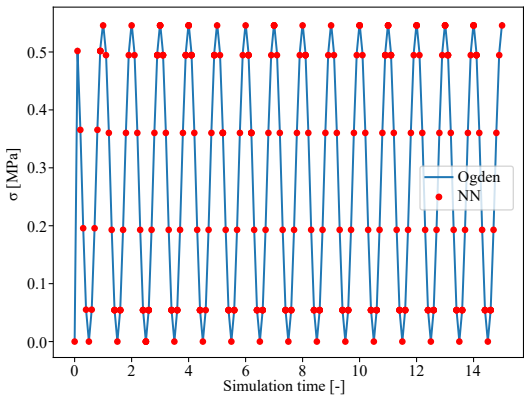
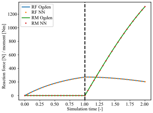
The central claim is that the damaged strain energy $\psi = (1-\zeta)\psi_0$ can be learned by a single feed-forward network whose undamaged block computes $\psi_0(I_1,I_2)$ from exponential activations $g(x)=e^{\alpha x}-1$ acting on weighted combinations of $I_1-3$ and $I_2-3$, while the same block, with shared weights, computes the historical maximum $\psi_{0,\max}$ that drives the damage parameter $\zeta = \zeta_\infty(1-e^{-\psi_{0,\max}/\iota})$. The network is trained on stresses only, obtained by automatic differentiation of the energy and the plane-stress Lagrange multiplier, so it never sees energy values during training and yet recovers energy and damage evolution. In the authors' tests the unconstrained variant (no polyconvexity constraints) reproduced the reference Ogden-with-Mullins model with median relative errors around 0.4% in the simple verification tests, about 0.9–1% in the rolling-disc boundary value problem, and about 0.4% in the diabolo tension–torsion problem.

Load-bearing premise

The weakest link is the assumption that stress data from three plane-stress tests determine the two-invariant strain energy and the damage law over every deformation state the network will later see, including the 3D states in the validation examples; the paper checks accuracy inside its training envelope but gives no proof that states outside it are recovered rather than extrapolated.

Editorial extensions

If this is right

If the claim holds, a constitutive model for a new rubber-like material with Mullins damage could be obtained from three standard laboratory tests, without postulating or calibrating a closed-form strain energy function.
The same network can be dropped into existing finite-element software through a UHYPER-style subroutine, since only energy derivatives with respect to invariants are needed.
The damage variable and the undamaged energy are recovered even though the network never sees energy or damage data during training, so the method extracts more from stress curves than a direct stress fit.
Dropping polyconvexity constraints gave the most accurate model in these tests, implying that strict convexity is not required for stable, accurate recovery on the tested domain.
The approach extends naturally to damage laws of unknown form by replacing the exponential damage expression with a small subnetwork whose output is bounded between 0 and 1.

Reading between the lines

Editorial extensions of the paper, not claims the author makes directly.

Editorial inference: the three training curves trace a two-dimensional surface in the $(I_1,I_2)$ plane, so the method should be understood as strong interpolation inside that envelope; its success on the disc and diabolo examples suggests the tested 3D states stayed within or near the trained region.
Editorial inference: a direct test of the method's boundary would be to run a 3D example whose deformation states clearly fall outside the $I_1 \le 50$, $I_2 \le 625$ envelope used for validation; if errors stay small there, the network is genuinely recovering the energy surface rather than interpolating it.
Editorial inference: the same architecture could be adapted to anisotropic damage by adding pseudo-invariants, which the authors note as a future direction; the subnetwork version of the damage law is the piece that makes this straightforward.
Editorial inference: because the network is trained on stress derivatives, its energy accuracy is only pinned at the undeformed state; a user who needs accurate total energies in large deformations should verify the recovered $\psi_0$ against calorimetric or independent data.

Share X Bluesky LinkedIn Reddit HN

Editorial analysis

A structured set of objections, weighed in public.

Desk editor's note, referee report, and a circularity audit.

Desk Editor's Note

read the letter

Colleague,

This is a solid methods paper on learning Mullins-type damage hyperelasticity with physics-augmented NNs. The core idea: a compact feed-forward energy network with an exponential activation, a shared-weight branch that computes the historical maximum undamaged energy, and a multiplicative damage factor. Trained on stress from three plane-stress tests (uniaxial, equibiaxial, planar tension), the network reproduces the generating Ogden-plus-Mullins model in 3D FEA benchmarks (rolling disc, diabolo) with median errors around 0.3–1.5%. That is a genuinely useful result for data-driven constitutive modeling, and the Abaqus implementation details are practical.

What is new: the shared-weight max-energy branch is a neat trick to let a network that only sees damaged stress still recover the undamaged backbone and damage evolution; the tanh subnetwork alternative and the comparison of six constraint cases are also useful. The paper is honest about a real identifiability issue: a trainable beta subnetwork can fit the stress data but get the energy and damage wrong (Fig. 14, Remarks 1–2). That is an important caveat, and they document it clearly.

The soft spots are real but mostly fixable. The abstract says the architecture fulfills polyconvexity and non-negativity, but the recommended case 4 enforces neither; the constrained cases underperform. That mismatch should be corrected in the abstract. More importantly, training and validation share the same synthetic Ogden generator, so there is no independent experimental test, though that is normal for a methods paper. The paper does not release code or trained weights, so the exact model is not reproducible from the text alone. Finally, the strongest claim—that three 1D plane-stress curves determine the full 2D energy and damage over the region reached in the 3D examples—is supported empirically but never checked directly: no invariant trajectory plots for the 3D integration points, so we do not know if those states fall inside the trained envelope or outside it. The random invariant-domain test (Fig. 13) helps, and the small 3D errors suggest the network is generalizing rather than extrapolating, but showing the actual invariant paths would close the gap.

Who is this for? Researchers working on neural constitutive models in computational mechanics, especially anyone wanting an FE-ready NN for rubber damage. It deserves serious peer review; a competent referee should ask for code/weights, the invariant-trajectory check, and a toned-down abstract. I would not desk-reject it.

Referee Report

4 major / 6 minor

Summary. The manuscript presents a physics-augmented feed-forward neural network for incompressible hyperelasticity with isotropic Mullins-type damage. The network outputs strain energy as a function of the invariants I1, I2 and of a maximum-history undamaged energy, with stress obtained by automatic differentiation; a damage branch multiplies the undamaged energy by (1−ζ), using either a specialised exponential saturation law or a trainable tanh subnetwork. Training data are synthetic uniaxial, equibiaxial, and planar tension stress-stretch curves with loading/unloading cycles, generated from a three-term Ogden model with damage (ζ∞=0.8, ι=1). Six constrained and unconstrained architecture variants are compared; the unconstrained network (case 4) gives the lowest loss and the best agreement in subsequent tests. The model is implemented in an Abaqus UHYPER subroutine and tested on homogeneous verification tests, a rolling solid rubber disc, and a diabolo under tension-torsion, with reported median errors mostly below 1.5% for stresses and reactions, and good qualitative agreement for damage evolution.

Significance. The practical aim — a compact, few-parameter neural-network constitutive model for incompressible rubber with Mullins damage, trained only on three plane-stress tests and usable in a commercial finite-element package — is attractive, and the paper provides a useful engineering recipe. Strengths include the complete UHYPER implementation details (Algorithms 1 and 2), a systematic comparison of six architecture/constraint cases, and quantitative error reporting on stresses, energies, reaction forces, and damage fields. The claim of 'full 3D recovery' is plausible but not fully established: the paper does not show that the 3D deformation states lie inside the trained invariant envelope, and the specialised damage branch partly assumes the generator's functional form. The paper's own Fig. 14 example demonstrates that stress data alone can admit models with wrong energy and damage, so the identifiability gap is real and should be addressed before the strongest conclusions are drawn.

major comments (4)

[Sec. 2.1, Sec. 4.2, Sec. 4.3] The central claim that three one-parameter training curves determine the full two-dimensional energy and damage evolution is not verified for the 3D examples. Training data are uniaxial, equibiaxial, and planar tension curves (Sec. 2.1); Fig. 13 validates the energy on a random invariant domain with I1≤50 and I2≤625, but the paper never reports the (I1,I2) states actually visited at integration points in the rolling-disc (Sec. 4.2) and diabolo (Sec. 4.3) simulations. If those states fall within the trained envelope, the examples are interpolation; if they fall outside, the conclusion that the network 'correctly captures the full 3D behaviour' rests on extrapolation. Please add invariant-trajectory plots for the 3D examples overlaid on Fig. 12, and report the maximum energy error along those trajectories.
[Sec. 3.1, Eq. (10)] The specialised damage branch uses the same exponential saturation law as the data generator (Eq. (10)), with ζmax and ι_NN trained. Consequently the agreement of ζ and energy in Figs. 11c, 22, and 27 confirms parameter identification within a known functional form rather than discovery of the damage law from data. Report the trained values of ζmax and ι_NN for the case-4 network and compare them with the generator values (0.8 and 1.0); this will clarify the epistemological status of the 'recovery' claimed in the abstract.
[Abstract, Sec. 3.2.1, Sec. 5] The abstract states that the architecture fulfils polyconvexity and non-negativity of the energy, but the recommended model is case 4 (Sec. 3.2.1), for which no weights are constrained and neither property is guaranteed. Sec. 3.2 explicitly relaxes the polyconvexity criteria, and the conclusion says overconstraining the network to be polyconvex is too restrictive. The abstract should be rephrased to distinguish the constraints enforced a priori (objectivity, thermodynamic consistency, normalisation) from properties that are only numerically observed (non-negativity) or not enforced (polyconvexity).
[Sec. 4.1.1, Fig. 14] The trainable-β subnetwork experiment is a load-bearing counterexample that deserves more discussion than a brief remark. It fits the stress curves with 4.3% error but mispredicts energy and damage for λ>5, with β=0.86 exceeding the generator's ζ∞=0.8. This demonstrates non-uniqueness of energy and damage given stress-only training data. The paper should either supply an identifiability argument for the specialised damage branch (e.g., that the exponential form plus shared weights removes the degeneracy), or add information (energy measurements, dissipation data, or additional loading paths) to justify the claimed recovery of energy and damage.

minor comments (6)

[Sec. 4.3.1] The paragraph begins with the typo 'In tIn this section'; please correct it.
[Sec. 1] The word 'refferred' should be 'referred'.
[Sec. 3.2.1] The word 'futlfilled' should be 'fulfilled'.
[Eq. (A.3)] The notation C_i is introduced in the brace in Eq. (A.3) but is not used elsewhere; the derivative expression is correct, but the brace annotation is unnecessary and could be removed.
[Fig. 13] The color map for relative error and the number of random samples used to create the invariant domain are not specified; please add a color bar and state the sample count.
[Algorithms 1 and 2] Algorithm 2 is referenced in the text but appears without a formal caption; label it consistently with Algorithm 1.

Circularity Check

1 steps flagged · score 4.0 of 10

Damage evolution is reported as a prediction but is produced by the same exponential saturation law used to generate the training data; the energy/3D recovery remains an independent fit.

fitted input called prediction [Sec. 2 Eq. (10); Sec. 2.1; Sec. 3.1 Fig. 5; Sec. 4.1 Fig. 11(c)]
"The damage parameter ζ is described with the expression ζ(γ) = ζ∞ ( 1−exp(−γ/ι) ) ... All of the data is generated using the Ogden material model with the constants from Table 1, ζ∞ = 0.8 and ι = 1. ... The calculation of the maximum strain energy and damage variable from Eq. (10) was added to the NN ... the trainable parameters in this NN are ... ζmax and ιNN when calculating the damage parameter ζ."

The training data are produced with Eq. (10) using ζ∞=0.8 and ι=1. The specialised damage branch in Fig. 5 implements exactly Eq. (10), with only ζmax and ιNN as trainable parameters. Consequently, the 'predicted' damage evolution shown in Fig. 11(c) (and used in the 3D examples) is not recovered independently from stress data; it is the same exponential saturation law as the generator, evaluated with fitted constants and with ψ0,max from the fitted energy subnetwork. The paper even states the form is 'taken from the literature' and offers the tanh subnetwork as a more general alternative, confirming that the specialised branch is an assumed ansatz.

full rationale

The central energy-recovery claim is not circular: the network is trained only on 2nd Piola-Kirchhoff stress data via Sobolev-style derivative loss, and the undamaged energy ψ0 is validated over an invariant domain (Fig. 13) and in 3D boundary-value problems against the same Ogden reference model. That is interpolation/verification, not reduction to the training data by construction. The one genuine circularity-like step is the damage branch: the specialised Mullins function used in the network is identical in form to the generator's damage law (Eq. (10)), so the reported damage evolution is a fitted version of the input assumption rather than an independent recovery. The paper partially mitigates this by testing a more general tanh subnetwork (Sec. 3.1.1 and Sec. 4.1.1), which does not assume the exponential saturation form and still captures the damage when β is omitted; this shows the method can work without the exact ansatz and keeps the central claim from collapsing entirely. The missing invariant-trajectory check for the 3D examples is a correctness/coverage concern, not circularity, and is excluded from the score. Self-citations (e.g., [11]) are descriptive and not load-bearing.

Assumptions & free parameters 5 free parameters · 6 assumptions · 0 invented entities

No new physical entities are introduced. The damage variable and the subnetworks are modelling constructs from existing theory. The ledger instead records the many fitted weights, the assumed damage law, the identifiability assumption about the three training curves, and the stability assumption of the unconstrained network.

free parameters (5)

NN weights w1,i, w2,i, w3,i, α_i (base energy block) = not reported
Fitted to 2nd Piola-Kirchhoff stress data via Adam; the hidden layer size n is not stated and final weights are not given.
damage parameters ζ_max and ι_NN (specialised damage function) = not reported
Trainable constants in Eq. (10) fitted to data generated with ζ∞=0.8 and ι=1; final values are not reported.
subnetwork weights and β (alternative damage model) = β = 0.86 when trainable
The 5-neuron tanh subnetwork fits β=0.86 to stress data, which the paper shows yields a wrong damage/energy split beyond λ=5; other subnetwork weights are not reported.
activation exponent initialisation α=0; ζ_max=1; ι=1; Glorot initialisation = initialisation values
Hyperparameter and initialisation choices that affect training success; α=0 is stated as necessary for convergence.
number of hidden neurons n (base NN) = unspecified
Architecture size chosen by hand and not reported, preventing exact reproduction of the results.

assumptions (6)

domain assumption Incompressibility J=det F=1, with I1≥3 and I2≥3; a Lagrange multiplier p handles the constraint.
Used throughout to define stress (Eqs. (2)-(7)) and to argue normalisation of stress and non-negativity of energy.
domain assumption Mullins damage is isotropic and described by ζ(γ)=ζ∞(1-exp(-γ/ι)) with γ=max ψ0.
This classical form from the literature (Eq. (10)) is assumed by the specialised damage branch; a real material with a different damage law would not be captured by that branch.
ad hoc to paper The three plane-stress deformation modes sample enough of the (I1,I2) domain to determine ψ0 and the damage evolution for the 3D cases.
Sec. 2.1 and Sec. 4 provide empirical support via Fig. 13 and the FEA examples, but no identifiability proof is given.
ad hoc to paper The unconstrained NN (case 4) remains material-stable in the FE examples even without polyconvexity.
Sec. 3.2.1 and Sec. 4: the recommended model drops the polyconvexity and non-negativity constraints; stability in the examples is observed, not guaranteed.
standard math The exponential activation g(x)=e^{αx}-1 with non-negative weights yields a polyconvex strain energy for the fully constrained case.
Composition rules for convex functions (Boyd and Vandenberghe) and Ball's polyconvexity theorems are invoked in Sec. 3 to justify case 1.
domain assumption TensorFlow automatic differentiation correctly computes the derivatives of the NN output for Sobolev training.
The custom loss in Sec. 3.2 uses autodiff to obtain stress from energy; the correctness of this tooling is assumed.

how reviews work

0 comments

Cite this review

Pith. "Pith review of Recovering Mullins damage hyperelastic behaviour with physics augmented neural networks." pith.science (2026). https://pith.science/paper/5ARNRA7A

@misc{pith2026241113185,
  author       = {Pith},
  title        = {Pith review of: Recovering Mullins damage hyperelastic behaviour with physics augmented neural networks},
  year         = {2026},
  howpublished = {\url{https://pith.science/paper/5ARNRA7A}},
  note         = {Machine review of arXiv:2411.13185}
}

read the original abstract

The aim of this work is to develop a neural network for modelling incompressible hyperelastic behaviour with isotropic damage, the so-called Mullins effect. This is obtained through the use of feed-forward neural networks with special attention to the architecture of the network in order to fulfil several physical restrictions such as objectivity, polyconvexity, non-negativity, material symmetry and thermodynamic consistency. The result is a compact neural network with few parameters that is able to reconstruct the hyperelastic behaviour with Mullinstype damage. The network is trained with artificially generated plane stress data and even correctly captures the full 3D behaviour with much more complex loading conditions. The energy and stress responses are correctly captured, as well as the evolution of the damage. The resulting neural network can be seamlessly implemented in widely used simulation software. Implementation details are provided and all numerical examples are performed in Abaqus.

Figures

Figures reproduced from arXiv: 2411.13185 by the authors.

**Figure 2.** Modes of deformation used during training. The imposed stretch is marked as [PITH_FULL_IMAGE:figures/full_fig_p010_2.png] view at source ↗

**Figure 3.** Stress-stretch plots of the 3 deformation cases, Cauchy stress shown. These [PITH_FULL_IMAGE:figures/full_fig_p011_3.png] view at source ↗

Figures from the paper (28 more)

**Figure 4.** Figure 4: Architecture of the basic FFNN used to model hyperelastic behaviour. This [PITH_FULL_IMAGE:figures/full_fig_p013_4.png]

**Figure 5.** Figure 5: Schematic of the expanded NN that takes into account the Mullins effect. The [PITH_FULL_IMAGE:figures/full_fig_p014_5.png]

**Figure 6.** Figure 6: Alternative subnetwork for modelling the damage parameter [PITH_FULL_IMAGE:figures/full_fig_p016_6.png]

**Figure 7.** Figure 7: NN block where the invariants are separated rather than added together under [PITH_FULL_IMAGE:figures/full_fig_p019_7.png]

**Figure 8.** Figure 8: Training results for the different cases of NNs. [PITH_FULL_IMAGE:figures/full_fig_p021_8.png]

**Figure 9.** Figure 9: Losses during training of the NN with a subnetwork for modelling the damage [PITH_FULL_IMAGE:figures/full_fig_p022_9.png]

**Figure 10.** Figure 10: Comparison of stress-stretch plots of the 3 deformation cases with the results [PITH_FULL_IMAGE:figures/full_fig_p024_10.png]

**Figure 11.** Figure 11: Plots of the strain energy, both with and without damage, and the damage [PITH_FULL_IMAGE:figures/full_fig_p025_11.png]

**Figure 12.** Figure 12: View of the invariant domain on which the energy is tested. Random samples [PITH_FULL_IMAGE:figures/full_fig_p026_12.png]

**Figure 13.** Figure 13: Relative error of the predicted Mullins energy over the invariant domain. [PITH_FULL_IMAGE:figures/full_fig_p026_13.png]

**Figure 14.** Figure 14: Results of Cauchy stress, damaged and undamaged energy, and damage param [PITH_FULL_IMAGE:figures/full_fig_p029_14.png]

**Figure 15.** Figure 15: Relative error of the predicted Mullins energy over the invariant domain. [PITH_FULL_IMAGE:figures/full_fig_p030_15.png]

**Figure 16.** Figure 16: Relative error of the predicted Mullins energy over the invariant domain. [PITH_FULL_IMAGE:figures/full_fig_p031_16.png]

**Figure 17.** Figure 17: Cyclic test with a constant amplitude, first 15 cycles shown for illustration, the [PITH_FULL_IMAGE:figures/full_fig_p032_17.png]

**Figure 18.** Figure 18: Cyclic test with progressively increasing loads, 20 loading cycles performed. [PITH_FULL_IMAGE:figures/full_fig_p032_18.png]

**Figure 19.** Figure 19: Solid rubber disc example from Abaqus. This is a simplified model of a vehicle [PITH_FULL_IMAGE:figures/full_fig_p033_19.png]

**Figure 20.** Figure 20: Reaction forces and moments at the central reference point at which the dis [PITH_FULL_IMAGE:figures/full_fig_p033_20.png]

**Figure 21.** Figure 21: Von Mises stress plots of the NN and referent solution, the absolute difference [PITH_FULL_IMAGE:figures/full_fig_p034_21.png]

**Figure 22.** Figure 22: Plots of damage variable ζ of the NN model and reference Ogden model. a body might be a quantity of interest. For comparison, the plots of the damage variables across the solid disc are given in [PITH_FULL_IMAGE:figures/full_fig_p035_22.png]

**Figure 23.** Figure 23: Reaction forces and moments at the central reference point at which the dis [PITH_FULL_IMAGE:figures/full_fig_p036_23.png]

**Figure 24.** Figure 24: Sketch of the diabolo geometry, fixed boundary condition and prescribed dis [PITH_FULL_IMAGE:figures/full_fig_p037_24.png]

**Figure 25.** Figure 25: Reaction force and moment at the node where displacement and rotation are [PITH_FULL_IMAGE:figures/full_fig_p038_25.png]

**Figure 26.** Figure 26: Von Mises stress plots of the diabolo problem using the proposed NN solution [PITH_FULL_IMAGE:figures/full_fig_p039_26.png]

**Figure 27.** Figure 27: Evolution of the damage variable ζ during simulation. The vertical dashed line represents the end of the uniaxial tension step and beginning of the torsional load step. hyperelastic behaviour in 3 dimensions. Also, it has been demonstrated that overconstraining the NN…

**Figure 28.** Figure 28: Plots of the damage variable values on the full diabolo geometry at the end of [PITH_FULL_IMAGE:figures/full_fig_p041_28.png]

**Figure 29.** Figure 29: Evolution of the strain energy for the whole model during simulation. The [PITH_FULL_IMAGE:figures/full_fig_p042_29.png]

**Figure 30.** Figure 30: Diabolo reaction force and moment at the node where the displacement and [PITH_FULL_IMAGE:figures/full_fig_p042_30.png]

**Figure 31.** Figure 31: Evolution of the damage variable ζ during simulation. Results shown for NNs with a subnetwork for modelling damage. The dashed vertical line marks the end of uniaxial tension step and beginning of torsional load step. Acknowledgements This work was supported in part b…

Discussion (0). Continue with ORCID to comment.

Reference graph

Works this paper leans on

39 extracted references · 17 canonical work pages

[1]

Kirchdoerfer, M

T. Kirchdoerfer, M. Ortiz, Data-driven computational mechanics, Com- puter Methods in Applied Mechanics and Engineering 304 (2016) 81–

work page 2016
[2]

Platzer, A

A. Platzer, A. Leygue, L. Stainier, M. Ortiz, Finite element solver for data-driven finite strain elasticity, Computer Methods in Applied Me- chanics and Engineering 379 (2021) 113756.doi:10.1016/j.cma.2021. 113756

doi:10.1016/j.cma.2021 2021
[3]

Eggersmann, T

R. Eggersmann, T. Kirchdoerfer, S. Reese, L. Stainier, M. Ortiz, Model- free data-driven inelasticity, Computer Methods in Applied Mechanics and Engineering 350 (2019) 81–99.doi:10.1016/j.cma.2019.02.016

doi:10.1016/j.cma.2019.02.016 2019
[4]

Bulin, J

J. Bulin, J. Hamaekers, M. Ariza, M. Ortiz, Interatomic-potential-free, data-driven molecular dynamics, Computer Methods in Applied Me- chanics and Engineering 415 (2023) 116224.doi:10.1016/j.cma.2023. 116224

doi:10.1016/j.cma.2023 2023
[5]

Karapiperis, L

K. Karapiperis, L. Stainier, M. Ortiz, J. Andrade, Data-driven multi- scale modeling in mechanics, Journal of the Mechanics and Physics of Solids 147 (2021) 104239.doi:10.1016/j.jmps.2020.104239

arXiv 2021
[6]

Mullins, Effect of stretching on the properties of rubber, Rubber Chemistry and Technology 21 (2) (1948) 281–300

L. Mullins, Effect of stretching on the properties of rubber, Rubber Chemistry and Technology 21 (2) (1948) 281–300. doi:10.5254/1. 3546914. 46

work page doi:10.5254/1 1948
[7]

Hornik, M

K. Hornik, M. Stinchcombe, H. White, Multilayer feedforward networks are universal approximators, Neural Networks 2 (5) (1989) 359–366. doi:10.1016/0893-6080(89)90020-8

doi:10.1016/0893-6080(89)90020-8 1989
[8]

Ghaboussi, J

J. Ghaboussi, J. H. Garrett, X. Wu, Knowledge-based modeling of ma- terial behavior with neural networks, Journal of Engineering Mechanics 117 (1) (1991) 132–153. doi:10.1061/(asce)0733-9399(1991)117: 1(132)

doi:10.1061/(asce)0733-9399(1991)117: 1991

Show all 39 references

[9]

Y.Shen, K.Chandrashekhara, W.F.Breig, L.R.Oliver, Neuralnetwork based constitutive model for rubber material, Rubber Chemistry and Technology 77 (2) (2004) 257–277.doi:10.5254/1.3547822

2004 doi
[10]

Weber, J

P. Weber, J. Geiger, W. Wagner, Constrained neural network train- ing and its application to hyperelastic material modeling, Com- putational Mechanics 68 (5) (2021) 1179–1204. doi:10.1007/ s00466-021-02064-8

2021
[11]

Zlatić, M

M. Zlatić, M. Čanađija, Incompressible rubber thermoelasticity: a neu- ral network approach, Computational Mechanics 71 (5) (2023) 895–916. doi:10.1007/s00466-023-02278-y

2023 doi
[12]

Huang, J

D. Huang, J. N. Fuhg, C. Weißenfels, P. Wriggers, A machine learn- ing based plasticity model using proper orthogonal decomposition, Computer Methods in Applied Mechanics and Engineering 365 (2020) 113008. doi:10.1016/j.cma.2020.113008

2020
[13]

Ghaderi, V

A. Ghaderi, V. Morovati, R. Dargazany, A physics-informed assembly of feed-forwardneuralnetworkenginestopredictinelasticityincross-linked polymers, Polymers 12 (11) (2020) 2628.doi:10.3390/polym12112628

2020 doi
[14]

Abdusalamov, J

R. Abdusalamov, J. Weise, M. Itskov, Rediscovering the Mullins ef- fect with deep symbolic regression (2024). arXiv:2403.05495, doi: 10.48550/ARXIV.2403.05495

2024 doi arXiv
[15]

Linka, M

K. Linka, M. Hillgärtner, K. P. Abdolazizi, R. C. Aydin, M. Itskov, C. J. Cyron, Constitutive artificial neural networks: A fast and gen- eral approach to predictive data-driven constitutive modeling by deep learning, Journal of Computational Physics 429 (2021) 110010. doi: 10...

2021
[16]

Thakolkaran, A

P. Thakolkaran, A. Joshi, Y. Zheng, M. Flaschel, L. De Lorenzis, S. Ku- mar, NN-EUCLID: Deep-learning hyperelasticity without stress data, Journal of the Mechanics and Physics of Solids 169 (2022) 105076. doi:10.1016/j.jmps.2022.105076

2022
[17]

D. K. Klein, M. Fernández, R. J. Martin, P. Neff, O. Weeger, Poly- convex anisotropic hyperelasticity with neural networks, Journal of the Mechanics and Physics of Solids 159 (2022) 104703.doi:10.1016/j. jmps.2021.104703

2022
[18]

Linden, D

L. Linden, D. K. Klein, K. A. Kalina, J. Brummund, O. Weeger, M. Kästner, Neural networks meet hyperelasticity: A guide to enforc- ing physics, Journal of the Mechanics and Physics of Solids 179 (2023) 105363. doi:10.1016/j.jmps.2023.105363

2023
[19]

F. Masi, I. Stefanou, P. Vannucci, V. Maffi-Berthier, Thermodynamics- based artificial neural networks for constitutive modeling, Journal of the Mechanics and Physics of Solids 147 (2021) 104277.doi:10.1016/j. jmps.2020.104277

2021
[20]

K. A. Kalina, L. Linden, J. Brummund, P. Metsch, M. Kästner, Auto- mated constitutive modeling of isotropic hyperelasticity based on artifi- cial neural networks, Computational Mechanics 69 (1) (2021) 213–232. doi:10.1007/s00466-021-02090-6

2021 doi
[21]

B. Amos, L. Xu, J. Z. Kolter, Input convex neural networks, in: D. Pre- cup, Y. W. Teh (Eds.), Proceedings of the 34th International Conference on Machine Learning, Vol. 70 of Proceedings of Machine Learning Re- search, PMLR, 2017, pp. 146–155

2017
[22]

D. K. Klein, F. J. Roth, I. Valizadeh, O. Weeger, Parametrized poly- convex hyperelasticity with physics-augmented neural networks, Data- Centric Engineering 4 (2023).doi:10.1017/dce.2023.21

2023 doi
[23]

K. A. Kalina, P. Gebhart, J. Brummund, L. Linden, W. Sun, M. Käst- ner, Neural network-based multiscale modeling of finite strain magneto- elasticity with relaxed convexity criteria, Computer Methods in Applied Mechanics and Engineering 421 (2024) 116739. doi:10.1016/j.cma. 20...

2024
[24]

N. N. Vlassis, R. Ma, W. Sun, Geometric deep learning for computa- tional mechanics Part I: anisotropic hyperelasticity, Computer Meth- ods in Applied Mechanics and Engineering 371 (2020) 113299. doi: 10.1016/j.cma.2020.113299

2020
[25]

N. N. Vlassis, W. Sun, Sobolev training of thermodynamic-informed neural networks for interpretable elasto-plasticity models with level set hardening, Computer Methods in Applied Mechanics and Engineering 377 (2021) 113695. doi:10.1016/j.cma.2021.113695

2021
[26]

W. M. Czarnecki, S. Osindero, M. Jaderberg, G. Swirszcz, R. Pascanu, Sobolev training for neural networks, in: I. Guyon, U. V. Luxburg, S. Bengio, H. Wallach, R. Fergus, S. Vishwanathan, R. Garnett (Eds.), Advances in Neural Information Processing Systems, Vol. 30, Curran Asso...

2017
[27]

Ogden, Large deformation isotropic elasticity – on the correlation of theory and experiment for incompressible rubberlike solids, Proceedings of the Royal Society of London

R. Ogden, Large deformation isotropic elasticity – on the correlation of theory and experiment for incompressible rubberlike solids, Proceedings of the Royal Society of London. A. Mathematical and Physical Sciences 326 (1567) (1972) 565–584.doi:10.1098/rspa.1972.0026

1972
[28]

J. M. Ball, Convexity conditions and existence theorems in nonlinear elasticity, Archive for rational mechanics and Analysis 63 (1976) 337– 403

1976
[29]

J. M. Ball, Constitutive inequalities and existence theorems in nonlin- ear elastostatics, in: Nonlinear analysis and mechanics: Heriot-Watt symposium, Vol. 1, Pitman London, 1977, pp. 187–241

1977
[30]

S. J. Connolly, D. Mackenzie, Y. Gorash, Isotropic hyperelasticity in principal stretches: explicit elasticity tensors and numerical imple- mentation, Computational Mechanics 64 (5) (2019) 1273–1288. doi: 10.1007/s00466-019-01707-1

2019 doi
[31]

Steinmann, M

P. Steinmann, M. Hossain, G. Possart, Hyperelastic models for rubber- like materials: consistent tangent operators and suitability for treloar’s data, Archive of Applied Mechanics 82 (9) (2012) 1183–1217. doi: 10.1007/s00419-012-0610-z. 49

2012 doi
[32]

K.Linka, E.Kuhl, Anewfamilyofconstitutiveartificialneuralnetworks towards automated model discovery, Computer Methods in Applied Me- chanics and Engineering 403 (2023) 115731.doi:10.1016/j.cma.2022. 115731

2023 doi
[33]

Diani, B

J. Diani, B. Fayolle, P. Gilormini, A review on the Mullins effect, European Polymer Journal 45 (3) (2009) 601–612. doi:10.1016/j. eurpolymj.2008.11.017

2009 doi
[34]

L. R. G. Treloar, Stress-strain data for vulcanised rubber under various types of deformation, Transactions of the Faraday Society 40 (1944) 59. doi:10.1039/tf9444000059

1944 doi
[35]

Glorot, Y

X. Glorot, Y. Bengio, Understanding the difficulty of training deep feed- forward neural networks, Journal of Machine Learning Research - Pro- ceedings Track 9 (2010) 249–256

2010
[36]

S. P. Boyd, L. Vandenberghe, Convex Optimization, Cambridge Univer- sity Press, 2004

2004
[37]

Abaqus 6.14 Analysis User’s Manual, Dassault Systemes Simulia, Inc., 2014

2014
[38]

Chagnon, E

G. Chagnon, E. Verron, G. Marckmann, L. Gornet, Development of new constitutive equations for the Mullins effect in rubber using the network alteration theory, International Journal of Solids and Structures 43 (22–23) (2006) 6817–6831.doi:10.1016/j.ijsolstr.2006.02.011. 50

2006 doi
[101]

doi:10.1016/j.cma.2016.02.001

2016 doi

Pith tools

Reviewed August 12, 2026 · model on record in the stance chip above.

[1] [1]

Kirchdoerfer, M

T. Kirchdoerfer, M. Ortiz, Data-driven computational mechanics, Com- puter Methods in Applied Mechanics and Engineering 304 (2016) 81–

work page 2016

[2] [2]

Platzer, A

A. Platzer, A. Leygue, L. Stainier, M. Ortiz, Finite element solver for data-driven finite strain elasticity, Computer Methods in Applied Me- chanics and Engineering 379 (2021) 113756.doi:10.1016/j.cma.2021. 113756

doi:10.1016/j.cma.2021 2021

[3] [3]

Eggersmann, T

R. Eggersmann, T. Kirchdoerfer, S. Reese, L. Stainier, M. Ortiz, Model- free data-driven inelasticity, Computer Methods in Applied Mechanics and Engineering 350 (2019) 81–99.doi:10.1016/j.cma.2019.02.016

doi:10.1016/j.cma.2019.02.016 2019

[4] [4]

Bulin, J

J. Bulin, J. Hamaekers, M. Ariza, M. Ortiz, Interatomic-potential-free, data-driven molecular dynamics, Computer Methods in Applied Me- chanics and Engineering 415 (2023) 116224.doi:10.1016/j.cma.2023. 116224

doi:10.1016/j.cma.2023 2023

[5] [5]

Karapiperis, L

K. Karapiperis, L. Stainier, M. Ortiz, J. Andrade, Data-driven multi- scale modeling in mechanics, Journal of the Mechanics and Physics of Solids 147 (2021) 104239.doi:10.1016/j.jmps.2020.104239

arXiv 2021

[6] [6]

Mullins, Effect of stretching on the properties of rubber, Rubber Chemistry and Technology 21 (2) (1948) 281–300

L. Mullins, Effect of stretching on the properties of rubber, Rubber Chemistry and Technology 21 (2) (1948) 281–300. doi:10.5254/1. 3546914. 46

work page doi:10.5254/1 1948

[7] [7]

Hornik, M

K. Hornik, M. Stinchcombe, H. White, Multilayer feedforward networks are universal approximators, Neural Networks 2 (5) (1989) 359–366. doi:10.1016/0893-6080(89)90020-8

doi:10.1016/0893-6080(89)90020-8 1989

[8] [8]

Ghaboussi, J

J. Ghaboussi, J. H. Garrett, X. Wu, Knowledge-based modeling of ma- terial behavior with neural networks, Journal of Engineering Mechanics 117 (1) (1991) 132–153. doi:10.1061/(asce)0733-9399(1991)117: 1(132)

doi:10.1061/(asce)0733-9399(1991)117: 1991