REVIEW 4 major objections 4 minor 64 references
A machine learning approach to estimate mid-infrared fluxes from WISE data
T0 review · 4 major / 4 minor · reviewed 2026-08-12 · deepseek-v4-flash
Pith's one-line read This paper claims that extremely randomized trees can predict Spitzer MIPS1 24 µm and IRAC4 8 µm fluxes from WISE fluxes and quality flags with $R^2 \approx 0.94$ and $R^2 \approx 0.98$, providing Spitzer-equivalent photometry across the…
desk verdict Solid held-out mapping of WISE to Spitzer fluxes, but the paper's real selling point—predicting Spitzer fluxes for sources without Spitzer detections—is never validated in that regime. read the letter →
The pith
A machine-rendered reading of the paper's core claim, the machinery that carries it, and where it could break.
The reading
What carries the argument
The central object is the extremely randomized trees (ET) regressor, an ensemble of decision trees in which both the feature subset and the split value at each node are chosen at random, with the final prediction obtained by averaging over trees. The pipeline first log-transforms the Spitzer target fluxes, applies Yeo-Johnson power transforms and standardization to the WISE predictors, selects relevant features with the Boruta algorithm, tunes hyperparameters through 10-fold cross-validation and randomized search, and estimates each prediction's 3σ uncertainty from the standard error of the individual tree predictions. This machinery carries the argument because it is what converts the noisy, partly contaminated WISE features into Spitzer-equivalent fluxes with small, well-characterized uncertainty intervals.
What would settle it
Take a set of allWISE sources that do have SEIP Spitzer detections but were not used in training because they are not open-cluster members or fail the clean-sample flags, apply the trained model, and compare predicted against measured 8 µm and 24 µm fluxes; if $R^2$ falls well below the reported 0.98 and 0.94 values, or if a systematic bias appears at fluxes below about $10^3$ µJy, the generalization claim fails.
Extended reading notes
Core claim
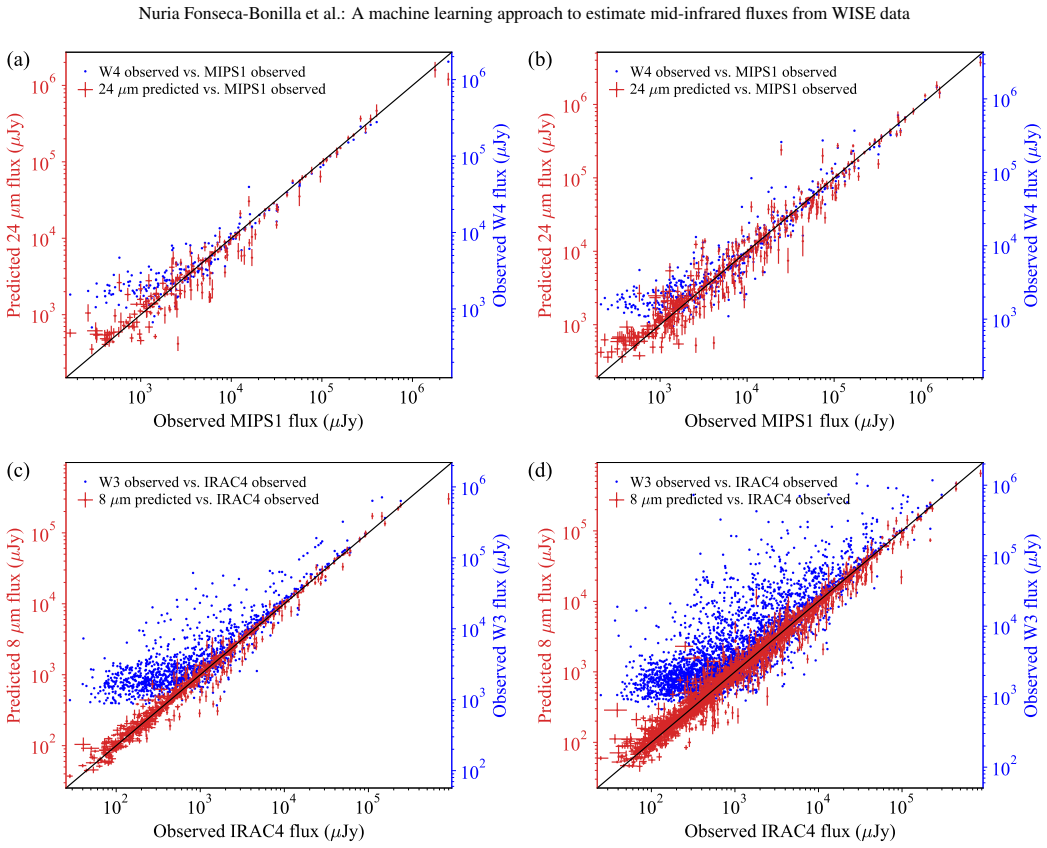
The central discovery is that a regression function learned from WISE variables can reproduce Spitzer mid-infrared fluxes closely enough to replace them for sources never observed by Spitzer. Using a training set of high-quality open cluster members with paired allWISE and SEIP data, extremely randomized trees predict MIPS1 24 µm fluxes with $R^2 \approx 0.94$ and IRAC4 8 µm fluxes with $R^2 \approx 0.98$, with mean absolute percentage errors below about 3.5%. The predicted fluxes stay close to the one-to-one line across the whole flux range, including the faint regime below roughly $10^3$ µJy where raw WISE W3 and W4 fluxes show the largest overestimations and scatter. The authors interpret this as evidence that the model captures hidden relationships between the two surveys, and that the approach can supply Spitzer-quality photometry for WISE-only sources while avoiding the massive data loss that stricter WISE quality cuts would incur.
Load-bearing premise
The method's generalization rests on the assumption that the WISE-to-Spitzer relationship learned from clean, high-quality open cluster members in the SEIP catalog holds for the broader allWISE population, including fainter, redder, or more embedded sources with SEIP counterparts.
Editorial extensions
If this is right
- For the clean-sample open cluster members without Spitzer detections, the model produces 24 µm fluxes for roughly 4,348 sources instead of discarding them, multiplying the usable sample about fourfold.
- At the faint end, where W4 and MIPS1 deviate by up to an order of magnitude, the ET predictions remain close to the diagonal, removing most of the scatter that plagues raw WISE photometry below about $10^3$ µJy.
- Because the learning curves show $R^2$ and MAPE improving monotonically with training-set size, retraining on larger future catalogs is expected to improve the predictions further.
- The ET models supply per-source 3σ uncertainty intervals from the spread across trees, with most relative errors below 10%, so the predicted fluxes can stand in for Spitzer data in SED fitting and infrared-excess searches.
- The approach avoids the data loss of conventional quality cuts: Appendix A shows that a signal-to-noise based selection would retain only about 508 to 650 useful sources, compared with thousands covered by the predicted fluxes.
Reading between the lines
- I would expect the trained model to transfer less cleanly to source populations absent from the open-cluster training set, such as heavily embedded young stellar objects or dusty galaxies; a direct validation on non-cluster SEIP sources with real Spitzer measurements would quantify the drop.
- The same pipeline could be applied to other overlapping survey pairs, for example predicting AKARI or IRAS mid-infrared fluxes from WISE, wherever the relationship between bandpasses is smooth enough for a regression model to learn.
- Because the paper reports a slight systematic overestimation below roughly $3\times 10^3$ µJy at 24 µm, users should treat individual faint predictions as statistically useful rather than exact fluxes, and should propagate the provided uncertainties when classifying disk-excess candidates.
- The feature-importance analysis suggests the 24 µm model relies on W4 at bright fluxes and switches to W3, W1, W2, and quality flags at faint fluxes; locating that switch threshold precisely could clarify the physical cause of the WISE-Spitzer discrepancy.
Editorial analysis
A structured set of objections, weighed in public.
Referee Report
Summary. The paper trains machine-learning regression models, specifically extremely randomized trees (ET), on a sample of open cluster members cross-matched between the SEIP Spitzer catalog and allWISE to predict Spitzer MIPS1 (24 um) and IRAC4 (8 um) fluxes from WISE W1-W4 fluxes and quality flags. The authors report coefficients of determination R2~0.94 for MIPS1 and R2~0.98 for IRAC4, compare ET to a linear baseline, perform feature selection with Boruta, and construct prediction uncertainties from the spread of tree predictions. They apply the trained models to sources without Spitzer detections and illustrate the results on spectral energy distributions of two members of IC 348. The claimed contribution is a method to obtain Spitzer-equivalent mid-infrared photometry over the WISE sky, particularly for faint sources where WISE and Spitzer disagree most.
Significance. If the method's accuracy extends to the unlabeled population, it would be a practically valuable tool: it would let investigators use the all-sky WISE catalog with photometry calibrated to Spitzer's higher resolution and sensitivity, and it explicitly targets the faint-flux regime where raw WISE photometry is most discrepant. The paper is also commendable for comparing against a linear baseline, reporting feature importances, and showing learning curves with training-set size. However, the significance is currently bounded by validation gaps: the headline metrics are cross-validation numbers on labeled sources, and the only external test is a two-star, hand-selected SED comparison in IC 348, so the method's usefulness for the intended no-detection application is asserted rather than demonstrated.
major comments (4)
- [Sec. 4.1, Table 2] The paper quotes R2~0.94 and R2~0.98 as the headline results, but the text states that the metrics in Table 2 'correspond to the average metrics obtained during the 10-fold cross-validation step,' not to predictions on the independently held-out test set. Section 3.2.1 reserves the test set for independent assessment and Fig. 5 shows test-set scatter, yet no test-set R2, MAPE, MAE, or RMSE are reported. Please report the test-set metrics explicitly and clarify whether the quoted R2 values are CV estimates or held-out test-set estimates; this distinction is central to the claim of predictive performance on sources not seen in training.
- [Sec. 3.2.1 and Fig. 3] Feature selection with Boruta is applied to the full labeled dataset before the train/test split. The workflow in Fig. 3 shows that the labeled dataset is used to select important features and that only afterward is the 'remaining training data' split into train and test sets. This leaks information from the test set into the feature choice, which can bias cross-validated performance estimates optimistically. Feature selection should be nested inside the cross-validation procedure, or at least performed on the training folds only, before the reported metrics are accepted as unbiased.
- [Sec. 4.2 and Fig. 2] The 'real-world' validation on IC 348 consists of two hand-selected stars, both of which have Spitzer detections and were chosen after an exploratory SED examination. This does not validate the main intended application: predicting fluxes for the roughly 80% of clean sources that lack MIPS1 measurements (Fig. 2). The convex-hull filter described in Sec. 2 ensures that unlabeled sources lie inside the WISE-feature envelope of the training set, but it does not guarantee that the conditional distribution of Spitzer flux given WISE features is the same for labeled and unlabeled sources. Please provide a quantitative check in the no-detection regime, for example by holding out a random subset of labeled sources and treating them as unlabeled, or by comparing predictions with Spitzer upper limits or an independent catalog.
- [Sec. 3.1.3] The uncertainty intervals are computed as three times the standard error of the mean of the individual tree predictions. Because trees in an ExtraTrees ensemble are not independent draws from a posterior distribution and the ensemble spread does not include irreducible noise, these intervals are likely to undercover the true flux uncertainty. For a method intended to identify infrared excesses, where error bars determine whether an excess is significant, a coverage calibration on the test set (e.g., the fraction of true fluxes within the reported 3-sigma intervals) should be reported or the uncertainty model should be revised.
minor comments (4)
- [Abstract and Sec. 4.2] There are several typographical errors: 'mid-infared' in the abstract, 'proofed reliable data' in Sec. 4.2, 'loosing data' in Sec. 5, and 'riveting solution' in Sec. 5 should be 'losing data' and 'attractive solution' (or similar).
- [Sec. 2, Fig. 2] The explanation of the count mismatch (e.g., 1096 sources with MIPS1 plus 4348 without does not sum to 9231) appears only in the body text; adding a sentence to the Fig. 2 caption about the convex-hull filtering step would make the figure self-explanatory.
- [Sec. 3.3.2] The description of the Boruta statistical test says features 'with probabilities below the confidence level alpha' are deemed irrelevant, which is the reverse of the usual Boruta decision rule; please clarify whether the intended criterion is that the feature importance is not significantly larger than the shadow features.
- [Sec. 4.1] The text says the Table 2 metrics are 'a pessimistic estimation' because the final model is retrained on train+test; this would be more convincing if the test-set metrics were shown alongside, particularly since the test-set scatter in Fig. 5 appears consistent with the CV values but no quantitative comparison is provided.
Circularity Check
No circularity: the regression result is evaluated on held-out data and the only self-references point to future applications, not to load-bearing premises.
full rationale
The paper is a supervised regression calibration: WISE features are inputs, Spitzer fluxes are targets, and performance is measured on a held-out 20% test set after k-fold cross-validation (Sections 3.2.1 and 4.1, Fig. 5). Because the test sources were not used in training or hyperparameter selection, the reported R2 ~ 0.94 (MIPS1) and R2 ~ 0.98 (IRAC4) are genuine out-of-sample accuracies rather than fits renamed as predictions. The IC 348 SED check is also external: those stars were not in the HR24 training sample, and the model predictions are compared to measured Spitzer fluxes (Section 4.2). No load-bearing claim is justified by a self-citation; the only self-references (footnote 1 and 'Fonseca-Bonilla et al. in prep.' in Section 4.2) point to future applications of the method, not to premises of the derivation. The authors explicitly disclaim physical prediction, stating that 'predict' is used in the statistical sense (Section 1). The convex-hull filtering and Boruta feature selection are applied before the train/test split and affect the training distribution, but this is a generalization caveat, not a circular reduction of the result to its inputs. No equation defines a target in terms of the output, and no fitted parameter is relabeled as a prediction.
Assumptions & free parameters
free parameters (6)
- Yeo-Johnson lambda_j per feature =
not reported per feature
- Standardization mean mu_j and std sigma_j per feature =
fitted on training folds
- ExtraTrees hyperparameters (n_trees, max_depth, min_samples_split, min_samples_leaf) =
chosen by randomized grid search (10-500 trees) with 10-fold CV
- Boruta confidence level alpha =
0.05
- Uncertainty confidence level =
3 sigma (99.7%)
- Train/test split ratio =
80/20
assumptions (5)
- domain assumption Spitzer SEIP fluxes are the true ground truth for 8 and 24 micron photometry.
- domain assumption The WISE-to-Spitzer relationship learned on open cluster members generalizes to other allWISE sources.
- standard math Decision tree predictions in ExtraTrees are sufficiently independent for CLT-based standard error.
- domain assumption Cross-match radius of 2 arcsec between HR24 and SEIP yields correct positional counterparts.
- standard math Boruta shadow-feature importance follows a binomial distribution under the null.
Cite this review
Pith. "Pith review of A machine learning approach to estimate mid-infrared fluxes from WISE data." pith.science (2026). https://pith.science/paper/OOEE56QI
@misc{pith2026241113321,
  author       = {Pith},
  title        = {Pith review of: A machine learning approach to estimate mid-infrared fluxes from WISE data},
  year         = {2026},
  howpublished = {\url{https://pith.science/paper/OOEE56QI}},
  note         = {Machine review of arXiv:2411.13321}
}
read the original abstract
While WISE is the largest, best quality infrared all-sky survey to date, a smaller coverage mission, Spitzer, was designed to have better sensitivity and spatial resolution at similar wavelengths. Confusion and contamination in WISE data result in discrepancies between them. We present a novel approach to work with WISE measurements with the goal of maintaining both its high coverage and vast amount of data while taking full advantage of the higher sensitivity and spatial resolution of Spitzer. We have applied machine learning (ML) techniques to a complete WISE data sample of open cluster members, using a training set of paired data from high-quality Spitzer Enhanced Imaging Products (SEIP), MIPS and IRAC, and allWISE catalogs, W1 (3.4 {\mu}m) to W4 (22 {\mu}m) bands. We have tested several ML regression models with the aim of predicting mid-infrared fluxes at MIPS1 (24 {\mu}m) and IRAC4 (8 {\mu}m) bands from WISE fluxes and quality flags. In addition, to improve the prediction quality, we have implemented feature selection techniques to remove irrelevant WISE variables. We have notably enhanced WISE detection capabilities, mostly at lowest magnitudes, which previously showed the largest discrepancies with Spitzer. In our particular case, extremely randomized trees was found to be the best algorithm to predict mid-infrared fluxes from WISE variables. We have tested our results in the SED of members of IC 348. We show discrepancies in the measurements of Spitzer and WISE and demonstrate the good concordance of our predicted fluxes with the real ones. ML is a fast and powerful tool that can be used to find hidden relationships between datasets, as the ones that exist between WISE and Spitzer fluxes. We believe this approach could be employed for other samples from the allWISE catalog with SEIP positional counterparts, and in other astrophysical studies with analogous discrepancies.
Figures


Figures from the paper (6 more)



Reference graph
Works this paper leans on
-
[1]
2020, PyCaret: An open source, low-code machine learning library in Python, pyCaret version 1.0.0
Ali, M. 2020, PyCaret: An open source, low-code machine learning library in Python, pyCaret version 1.0.0
work page 2020
-
[2]
Antoniucci, S., Giannini, T., Li Causi, G., & Lorenzetti, D. 2014, ApJ, 782, 51
work page 2014
-
[3]
Ball, N. M. & Brunner, R. J. 2010, International Journal of Modern Physics D, 19, 1049
work page 2010
- [4]
-
[5]
2008, A&A, 492, 277
Bayo, A., Rodrigo, C., Barrado Y Navascués, D., et al. 2008, A&A, 492, 277
2008
-
[6]
Beichman, C. A. 1988, Astrophysical Letters and Communications, 27, 67
work page 1988
- [7]
-
[8]
1994, Mixture density networks, Tech
Bishop, C. 1994, Mixture density networks, Tech. rep., Aston University
work page 1994
Show all 64 references
-
[9]
Bishop, C. M. 2007, Pattern Recognition and Machine Learning, 1st edn. (Springer)
2007
-
[10]
2001, Machine Learning, 45, 5
Breiman, L. 2001, Machine Learning, 45, 5
2001
-
[11]
J., & Olshen, R
Breiman, L., Friedman, J., Stone, C. J., & Olshen, R. 1984, Classification and Regression Trees (Chapman and Hall/CRC)
1984
-
[12]
J., Noriega-Crespo, A., Mizuno, D
Carey, S. J., Noriega-Crespo, A., Mizuno, D. R., et al. 2009, PASP, 121, 76
2009
-
[13]
& Sahin, F
Chandrashekar, G. & Sahin, F. 2014, Computers & Electrical Engineering, 40, 16, 40th-year commemorative issue 6 When applying this method to other samples or astrophysical studies, much care must be taken with their specific characteristics
2014
-
[14]
O., Scaife, A
Clarke, A. O., Scaife, A. M. M., Greenhalgh, R., & Griguta, V . 2020, A&A, 639, A84
2020
-
[15]
M., Wright, E
Cutri, R. M., Wright, E. L., Conrow, T., et al. 2013, Explanatory Supplement to the AllWISE Data Release Products, Explanatory Supplement to the All- WISE Data Release Products, by R. M. Cutri et al
2013
-
[16]
H., Hoard, D
Debes, J. H., Hoard, D. W., Kilic, M., et al. 2011, ApJ, 729, 4
2011
-
[17]
P., & Debes, J
Dennihy, E., Farihi, J., Gentile Fusillo, N. P., & Debes, J. H. 2020, ApJ, 891, 97
2020
-
[18]
2020, A&A, 634, A57
Dobbels, W., Baes, M., Viaene, S., et al. 2020, A&A, 634, A57
2020
-
[19]
Y ., et al
Duan, T., Avati, A., Ding, D. Y ., et al. 2020, NGBoost: Natural Gradient Boosting for Probabilistic Prediction
2020
-
[20]
& Tibshirani, R
Efron, B. & Tibshirani, R. J. 1993, An Introduction to the Bootstrap, Mono- graphs on Statistics and Applied Probability No. 57 (Boca Raton, Florida, USA: Chapman & Hall/CRC)
1993
-
[21]
Fluke, C. J. & Jacobs, C. 2020, WIREs Data Mining and Knowledge Discovery, 10, e1349 Gaia Collaboration, Brown, A. G. A., Vallenari, A., et al. 2018, A&A, 616, A1
2020
-
[22]
P., Mather, J
Gardner, J. P., Mather, J. C., Clampin, M., et al. 2006, Space Sci. Rev., 123, 485
2006
-
[23]
S., Cope, D., Ip, J., et al
Geiger, R. S., Cope, D., Ip, J., et al. 2021, Quantitative Science Studies, 2, 795
2021
-
[24]
2006, Machine Learning, 63, 3
Geurts, P., Ernst, D., & Wehenkel, L. 2006, Machine Learning, 63, 3
2006
-
[25]
Glass, I. S. 1999, Handbook of Infrared Astronomy
1999
-
[26]
2022, MNRAS, 517, 1837
Guo, X., Liu, C., Qiu, B., et al. 2022, MNRAS, 517, 1837
2022
-
[27]
R., Millman, K
Harris, C. R., Millman, K. J., van der Walt, S. J., et al. 2020, Nature, 585, 357
2020
-
[28]
2009, The elements of statistical learn- ing: data mining, inference and prediction, 2nd edn
Hastie, T., Tibshirani, R., & Friedman, J. 2009, The elements of statistical learn- ing: data mining, inference and prediction, 2nd edn. (Springer)
2009
-
[29]
Hunt, E. L. & Reffert, S. 2023, A&A, 673, A114
2023
-
[30]
Hunt, E. L. & Reffert, S. 2024, A&A, 686, A42 Ivezi´c, Ž., Connolly, A., Vanderplas, J., & Gray, A. 2019, Statistics, Data Mining and Machine Learning in Astronomy, 1st edn. (Princeton University Press)
2024
-
[31]
2017, in Advances in Neural Information Processing Systems, ed
Ke, G., Meng, Q., Finley, T., et al. 2017, in Advances in Neural Information Processing Systems, ed. I. Guyon, U. V . Luxburg, S. Bengio, H. Wallach, R. Fergus, S. Vishwanathan, & R. Garnett, V ol. 30 (Curran Associates, Inc.)
2017
-
[32]
Kennedy, G. M. & Wyatt, M. C. 2012, MNRAS, 426, 91
2012
-
[33]
F., Steinz, J
Kessler, M. F., Steinz, J. A., Anderegg, M. E., et al. 1996, A&A, 315, L27
1996
-
[34]
2016, A&A, 596, A39
Krakowski, T., Małek, K., Bilicki, M., et al. 2016, A&A, 596, A39
2016
-
[35]
S., & Igel, C
Kremer, J., Stensbo-Smidt, K., Gieseke, F., Pedersen, K. S., & Igel, C. 2017, IEEE Intelligent Systems, 32, 16
2017
-
[36]
2016, A&A, 592, A25
Kurcz, A., Bilicki, M., Solarz, A., et al. 2016, A&A, 592, A25
2016
-
[37]
Kursa, M. B. & Rudnicki, W. R. 2010, Journal of Statistical Software, 36, 1–13
2010
-
[38]
Lindholm, A., Wahlström, N., Lindsten, F., & Schön, T. B. 2022, Machine Learn- ing - A First Course for Engineers and Scientists (Cambridge University Press)
2022
-
[39]
2019, MNRAS, 487, 2522
Marton, G., Ábrahám, P., Szegedi-Elek, E., et al. 2019, MNRAS, 487, 2522
2019
-
[40]
2023, Reports on Progress in Physics, 86, 076901
Moriwaki, K., Nishimichi, T., & Yoshida, N. 2023, Reports on Progress in Physics, 86, 076901
2023
-
[41]
2007, PASJ, 59, S369
Murakami, H., Baba, H., Barthel, P., et al. 2007, PASJ, 59, S369
2007
-
[42]
Neal, R. M. 2012, Bayesian learning for neural networks, V ol. 118 (Springer Science & Business Media)
2012
-
[43]
J., van Duinen, R., et al
Neugebauer, G., Habing, H. J., van Duinen, R., et al. 1984, ApJ, 278, L1
1984
-
[44]
2018, Astronomy and Com- puting, 23, 72
Nguyen, T., Pankratius, V ., Eckman, L., & Seager, S. 2018, Astronomy and Com- puting, 23, 72
2018
-
[45]
2000, A&AS, 143, 23 pandas development team, T
Ochsenbein, F., Bauer, P., & Marcout, J. 2000, A&AS, 143, 23 pandas development team, T. 2020, pandas-dev/pandas: Pandas
2000
-
[46]
I., Metchev, S
Patel, R. I., Metchev, S. A., & Heinze, A. 2014, ApJS, 212, 10
2014
-
[47]
I., Metchev, S
Patel, R. I., Metchev, S. A., Heinze, A., & Trollo, J. 2017, AJ, 153, 54
2017
-
[48]
2018, High-Quality Prediction Intervals for Deep Learning: A Distribution-Free, Ensembled Approach
Pearce, T., Zaki, M., Brintrup, A., & Neely, A. 2018, High-Quality Prediction Intervals for Deep Learning: A Distribution-Free, Ensembled Approach
2018
-
[49]
2011, Journal of Machine Learning Research, 12, 2825
Pedregosa, F., Varoquaux, G., Gramfort, A., et al. 2011, Journal of Machine Learning Research, 12, 2825
2011
-
[50]
Z., Pesenson, I
Pesenson, M. Z., Pesenson, I. Z., & McCollum, B. 2010, Advances in Astron- omy, 2010, 350891
2010
-
[51]
M., Stapelfeldt, K
Rebull, L. M., Stapelfeldt, K. R., Evans, N. J., I., et al. 2007, ApJS, 171, 447
2007
-
[52]
& Röttgering, H
Retana-Montenegro, E. & Röttgering, H. J. A. 2020, A&A, 636, A12
2020
-
[53]
& Rokach, L
Sagi, O. & Rokach, L. 2018, WIREs Data Mining and Knowledge Discovery, 8, e1249
2018
-
[54]
& Serjeant, S
Sedgwick, C. & Serjeant, S. 2022, MNRAS, 515, 4828
2022
-
[55]
E., Evans, N
Shu, Y ., Koposov, S. E., Evans, N. W., et al. 2019, MNRAS, 489, 4741
2019
-
[56]
M., Kuchner, M
Silverberg, S. M., Kuchner, M. J., Wisniewski, J. P., et al. 2018, ApJ, 868, 43
2018
-
[57]
T., Korn, A
Suazo, M., Zackrisson, E., Wright, J. T., Korn, A. J., & Huston, M. 2022, MN- RAS, 512, 2988 van der Marel, N., Verhaar, B. W., van Terwisga, S., et al. 2016, A&A, 592, A126
2022
-
[58]
E., et al
Virtanen, P., Gommers, R., Oliphant, T. E., et al. 2020, Nature Methods, 17, 261
2020
-
[59]
W., Roellig, T
Werner, M. W., Roellig, T. L., Low, F. J., et al. 2004, ApJS, 154, 1 Wes McKinney. 2010, in Proceedings of the 9th Python in Science Conference, ed. Stéfan van der Walt & Jarrod Millman, 56 – 61
2004
-
[60]
L., Eisenhardt, P
Wright, E. L., Eisenhardt, P. R. M., Mainzer, A. K., et al. 2010, AJ, 140, 1868
2010
-
[61]
2020, ApJ, 902, 127
Xu, S., Lai, S., & Dennihy, E. 2020, ApJ, 902, 127
2020
-
[62]
& Johnson, R
Yeo, I.-K. & Johnson, R. A. 2000, Biometrika, 87, 954
2000
-
[63]
Z., Hafezianzadeh, F., Zhang, Y ., et al
Zeraatgari, F. Z., Hafezianzadeh, F., Zhang, Y ., et al. 2024, MNRAS, 527, 4677
2024
-
[64]
cleaning
Zhao, G., Qiu, B., Luo, A. L., et al. 2023, Research in Astronomy and Astro- physics, 23, 085010 Article number, page 12 of 13 Nuria Fonseca-Bonilla et al.: A machine learning approach to estimate mid-infrared fluxes from WISE data Appendix A: Data selection through WISE quali...
2012
Reviewed August 12, 2026 · model on record in the stance chip above.
Discussion (0). Continue with ORCID to comment.