REVIEW 3 major objections 6 minor 21 references
'Weather' in the LSST Camera: Investigating Patterns in Differenced Flat Images
T0 review · 3 major / 6 minor · reviewed 2026-08-12 · deepseek-v4-flash
Pith's one-line read The 'weather' pattern in LSST Camera flats is internal air turbulence, and simulations set its PSF effect at about one part in 10^4.
desk verdict Real flat-field systematic, convincingly traced to the purge system, but the PSF impact estimate is less precise than the abstract claims and the simulation's screen location does not match the paper's own physical inference. read the letter →
The pith
A machine-rendered reading of the paper's core claim, the machinery that carries it, and where it could break.
The reading
What carries the argument
The load-bearing object is a single phase screen: a thin plane of optical-path difference placed between lenses L1 and L2 in the simulation, standing in for the integrated effect of the turbulent air along the line of sight. It is a Gaussian random field with power spectrum $P(k) = A\,k^2\,(1+(k/k_c)^{5/2})^{-1}$, with fitted parameters $A = 0.5\ \mathrm{pix}^{-3}$ and $k_c = 5\ \mathrm{pix}^{-1}$, chosen so that simulated differenced flats match the peak-to-valley contrast and the correlation plateau of the real images. The 2-D correlation function of differenced flats is the matching diagnostic that connects observation and simulation; once the screen is matched, it is inserted into end-to-end ray-tracing simulations of the full LSST optical system, including atmospheric phase screens, telescope mirrors, camera lenses, and detector response, to measure the adaptive-moment PSF size across the focal plane for many simulated stars.
What would settle it
Run the LSST Camera, or a converging-beam laboratory copy of its optics, with the Volume Purge Cabinet alternating between on and off while measuring the adaptive-moment size of a point source; if the average PSF size shifts by more than about one part in $10^4$, the fitted phase-screen model underestimates the weather's impact.
Extended reading notes
Core claim
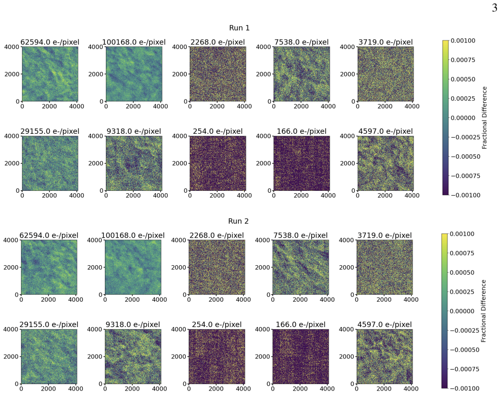
The core claim of the paper is that the 'weather' seen in differenced flat images of the LSST Camera during electro-optical testing comes from air turbulence inside the camera body, driven by the Volume Purge Cabinet that blows dry air over the lenses to prevent frost. Differences in air density change the index of refraction and slightly deflect light from the test projector, producing swirling fractional variations at the $10^{-3}$ level in flat pairs; the test stood out because it used diverging light, a large effective focal ratio, and sub-second LED flashes, all of which amplify sensitivity to air movement. The evidence for the mechanism is that the 2-D correlation functions of the patterns change with purge fan speed and change dramatically with the purge off, when stream-like features appear from the side opposite the purge nozzles. The quantitative conclusion comes from fitting a single phase screen between lenses L1 and L2 with a turbulence power spectrum that reproduces the observed correlations, then placing that screen in full simulations of the telescope and camera: the PSF size changes by about one part in $10^4$, and the authors state the weather 'should not affect the LSST.'
Load-bearing premise
The simulation rests on the assumption that a single thin phase screen between two lenses, with its strength tuned to match the observed flat-field correlations, faithfully represents the real three-dimensional air turbulence; if the turbulence is distributed differently along the light path, the same flat images could imply a different PSF effect.
Editorial extensions
If this is right
- During LSST operations, calibration flats taken with the converging $f/1.2$ beam and longer exposures should show the weather far more weakly than in the test-bench images, so no new calibration correction is required.
- The 2-D correlation function of flat pairs serves as a live monitor of the camera's internal air environment, clearly distinguishing purge fan settings and the purge-off state.
- The wings of the PSF beyond roughly 2.5 pixels are the part of the star image most sensitive to this kind of phase error, which is the region relevant to high-precision shape measurements.
- Test stands that illuminate with diverging beams and short flashes will continue to see this weather and should treat it as a known source of low-level structure in flat pairs.
- If the phase screen is a faithful model, the purge-induced air turbulence will be present during the survey at an amplitude too low to require PSF model terms.
Reading between the lines
- A direct confirmation the paper does not carry out would be to measure the LSST Camera PSF with the purge system toggled off, looking for a size shift at the $10^{-4}$ level; this would test the phase-screen extrapolation in situ.
- The fitted phase screen does not uniquely determine where along the light path the turbulence sits, and the PSF impact depends on that location, so the same flat images could in principle imply a larger effect.
- The same 2-D correlation technique could be adopted as a standard diagnostic for internal 'dome seeing' in any wide-field camera with a purge or thermal-control airflow system.
- Because the suppression comes from the speed of the $f/1.2$ beam, future instruments with slower internal beams may inherit a larger weather effect on the PSF, and the scaling with focal ratio is a natural next calculation.
Editorial analysis
A structured set of objections, weighed in public.
Referee Report
Summary. The paper reports a low-amplitude (10^-3 peak-to-peak) turbulent pattern in differenced flat-field images taken during electro-optical testing of the fully integrated LSST Camera with the CCOB Wide Beam projector. The authors characterize the pattern with 2-D correlation functions, show that it changes between exposures, and demonstrate through a VPC on/off comparison that the pattern is affected by the internal Volume Purge Cabinet. They attribute the effect to index-of-refraction variations in air inside the camera body, enhanced by the diverging, fast-ratio CCOB illumination geometry and short LED flashes. Using batoid and galsim, they fit a Gaussian random-field phase screen with a Kolmogorov-like power spectrum to reproduce the observed correlation plateau, place this screen between L1 and L2 in a full-telescope simulation, and conclude that the weather changes the PSF dispersion at the 10^-4 level, implying no impact on LSST.
Significance. If the conclusion holds, the paper is valuable in two ways. It identifies and explains a subtle environment-dependent systematic in lab flat-fielding for large cameras, and it quantitatively retires a potential concern about purge-system air turbulence for the LSST survey. The observational core is strong: the pattern is reproduced in many images, the full focal-plane mosaic shows coherent structure, and the VPC on/off comparison produces a clear structural change from swirls to stream-like patterns. The use of community-standard tools (galsim, batoid, TreeCorr) with the simulation parameters provided in the appendix aids reproducibility. The main quantitative claim about the PSF, however, is currently conditional on a fitted single phase screen at a location that appears inconsistent with the paper's own physical inference, and the reported statistics do not support a measured 10^-4 deterioration.
major comments (3)
- [Sec. 4 and Sec. 5] The phase screen used for the PSF-impact simulation is placed 'in between L1 and L2' (Sec. 4), but the paper's evidence places the VPC-driven air flow near L3: Sec. 3.1 says the structure is 'possibly close to the L3 where the VPC nozzle exists' and Sec. 5 states the VPC 'supplies air between the L3 and L2 lenses (air side).' For a fast f/1.2 converging beam, the induced wavefront error and its mapping to pupil coordinates depend on the axial location of the screen, so a screen calibrated under the diverging CCOB geometry at L1-L2 cannot be assumed to represent the L3-L2 location in the full telescope. Please repeat the simulation with the screen at the physically indicated location, or with a distributed screen along the air path, and show that the 10^-4 conclusion is unchanged.
- [Sec. 4 and Fig. 9] The statistical support for the headline number is not yet quantitative. For the 100-star run, the PSF sigma means are 1.0715 ± 0.005 (weather) and 1.0710 ± 0.005 (no weather); the 0.0005 difference is an order of magnitude smaller than the reported scatter, so the two cases are statistically indistinguishable. The single-star, 100-realization run gives 1.072 ± 0.001 in both cases. The conclusion in Sec. 5 that the PSF 'only deteriorate[s] by 10^-4' should be restated as an upper limit at about the 10^-4–10^-3 level unless a statistically significant difference can be demonstrated, and the increased-weather run should be used to calibrate the sensitivity.
- [Sec. 4, Eq. (2)] The PSF-impact prediction depends on the fitted phase-screen parameters A and k_c, together with the additional Gaussian smoothing scale, which are adjusted by hand until the simulated 2-D correlation 'plateau of 5 < r < 100 pixels' matches the observed one. Since the same fitted screen is then used to compute the PSF effect, the final number inherits the full uncertainty of that fit, including degeneracies among A, k_c, and the screen location. Please provide a sensitivity analysis (e.g., vary A and k_c by factors around the adopted values and report the resulting PSF sigma changes) so that the 10^-4 claim can be assessed independently of the tuning.
minor comments (6)
- [Fig. 5 caption] The caption notes that 'Only five exposures were taken at the lower fan speed.' This should be stated in the main text, since it limits any conclusion about fan speed; the VPC on/off contrast remains the strongest evidence for the attribution.
- [Sec. 3.1] The sentence 'The increase in the length of the plateau ... likely due to the large streak-like patterns' is a post hoc explanation; consider quantifying the correlation length to support this interpretation.
- [Abstract and Sec. 5] The abstract and conclusion use 'one part in 10^-4 level' and '10^-4' interchangeably; given the statistical scatter, please specify whether this is an upper limit or a measured value.
- [Eq. (2)] Please define the units of wavenumber k explicitly near the equation; the text later gives k_c = 5 pix^-1, but the convention for k in the power spectrum is not stated at first use.
- [Fig. 3 and Fig. 4] The color scale is not shown on either figure; please add it, as the 'peak-to-peak variations of a factor of 10^-3' claim otherwise cannot be read off the figures.
- [References] Reference [21] lists 'Ustumi, Y.'; this should be 'Utsumi, Y.'
Circularity Check
No circularity: the weather pattern is directly observed, the VPC attribution rests on controlled fan-speed comparisons, and the PSF impact estimate is a forward simulation from an explicitly fitted phase screen, not a prediction forced by the fit.
full rationale
The paper's primary empirical claim is the existence, structure, and VPC dependence of the weather pattern in differenced flat images; this is established by direct imaging (Figures 3, 4, 6) and by controlled changes of the VPC fan speed that visibly alter the 2D correlation functions (Figure 5), not by any fitted model. The central quantitative claim is the PSF impact estimate: a phase screen with power spectrum P(k)=A k^2 (1+(k/kc)^2)^(-5/2) is tuned so that simulated CCOB flat differences match the observed peak-to-peak variations and the 2D correlation plateau, and then that same screen is propagated through a batoid/galsim model of the full f/1.2 optical system. This is a legitimate forward-modeling chain: the screen parameters (A=0.5 pix^-3, kc=5 pix^-1) are fitted to the flat-field data, but the resulting PSF sigma difference of ~1e-4 is a new computed output, not a restatement of the fitted correlation function. The fit did not constrain the PSF impact to be small; a larger impact would have been possible if the optics amplified the screen. The paper explicitly acknowledges the modeling assumption of a single phase screen ('we make an assumption that a single phase screen can represent the weather') and the uncertainty in its axial placement (the physical evidence points near L3 while the simulation places the screen between L1 and L2); these are model-validity and calibration concerns, not circularity. Self-citations to batoid, EO-testing papers, and sensor-characterization papers are normal and are not load-bearing for the derivation: the simulation codes and prior test descriptions are independent tools, and the conclusion does not depend on an unverified self-cited uniqueness theorem. No step in the derivation reduces by construction to its own input.
Assumptions & free parameters
free parameters (3)
- A =
0.5 pix^-3
- k_c =
5 pix^-1
- Gaussian smoothing scale =
not explicitly given
assumptions (4)
- domain assumption The turbulent pattern can be represented by a single thin phase screen between L1 and L2
- ad hoc to paper The turbulence power spectrum has the functional form P(k) = A k^2 (1 + (k/k_c)^{5/2})^-1
- domain assumption The average of 1100 stability flat images is a weather-free reference
- domain assumption The weather pattern is frozen during the 0.9 s LED flash
Cite this review
Pith. "Pith review of 'Weather' in the LSST Camera: Investigating Patterns in Differenced Flat Images." pith.science (2026). https://pith.science/paper/HRGCGFY2
@misc{pith2026241113386,
  author       = {Pith},
  title        = {Pith review of: 'Weather' in the LSST Camera: Investigating Patterns in Differenced Flat Images},
  year         = {2026},
  howpublished = {\url{https://pith.science/paper/HRGCGFY2}},
  note         = {Machine review of arXiv:2411.13386}
}
read the original abstract
During electro-optical testing of the camera for the upcoming Vera C. Rubin Observatory Legacy Survey of Space and Time, a unique low-signal pattern was found in differenced pairs of flat images used to create photon transfer curves, with peak-to-peak variations of a factor of 10^-3. A turbulent pattern of this amplitude was apparent in many differenced flat-fielded images. The pattern changes from image to image and shares similarities with atmospheric 'weather' turbulence patterns. We applied several strategies to determine the source of the turbulent pattern and found that it is representative of the mixing of the air and index of refraction variations caused by the internal camera purge system displacing air, which we are sensitive to due to our flat field project setup. Characterizing this changing environment with 2-D correlation functions of the 'weather' patterns provides evidence that the images reflect the changes in the camera environment due to the internal camera purge system. Simulations of the full optical system using the galsim and batoid codes show that the weather pattern affects the dispersion of the camera point-spread function at only the one part in 10^-4 level
Figures


Figures from the paper (7 more)


Reference graph
Works this paper leans on
-
[1]
2019, A&A, 629, A36, doi: 10.1051/0004-6361/201935508
Astier, P., Antilogus, P., Juramy, C., et al. 2019, A&A, 629, A36, doi: 10.1051/0004-6361/201935508
-
[2]
2019, in Astronomical Society of the Pacific Conference Series, V ol
Bosch, J., AlSayyad, Y ., Armstrong, R., et al. 2019, in Astronomical Society of the Pacific Conference Series, V ol. 523, Astronomical Data Analysis Software and Systems XXVII, ed. P. J. Teuben, M. W. Pound, B. A. Thomas, & E. M. Warner, 521, doi: 10.48550/arXiv.1812.03248
-
[3]
Broughton, A., Utsumi, Y ., Plazas Malag´on, A. A., et al. 2024, PASP, 136, 045003, doi: 10.1088/1538-3873/ad3aa2
-
[4]
H., Utsumi, Y ., Snyder, A., et al
Esteves, J. H., Utsumi, Y ., Snyder, A., et al. 2023, PASP, 135, 115003, doi: 10.1088/1538-3873/ad0a73
-
[5]
2003, MNRAS, 343, 459, doi: 10.1046/j.1365-8711.2003.06683.x
Hirata, C., & Seljak, U. 2003, MNRAS, 343, 459, doi: 10.1046/j.1365-8711.2003.06683.x
arXiv 2003
-
[6]
2018, The LSST System Science Requirements Document, Tech
Ivezi´c, ˇZ., & the LSST Science Collaboration. 2018, The LSST System Science Requirements Document, Tech. rep., LSST-DA. https://docushare.lsst.org/docushare/dsweb/Get/LPM-17
work page 2018
-
[7]
Ivezi´c, ˇZ., Kahn, S. M., Tyson, J. A., et al. 2019, ApJ, 873, 111, doi: 10.3847/1538-4357/ab042c
-
[8]
Janesick, J. R. 2001, Scientific charge-coupled devices
work page 2001
Show all 21 references
-
[9]
2004, MNRAS, 352, 338, doi: 10.1111/j.1365-2966.2004.07926.x
Jarvis, M., Bernstein, G., & Jain, B. 2004, MNRAS, 352, 338, doi: 10.1111/j.1365-2966.2004.07926.x
2004
-
[10]
V ., Haupt, J., O’Connor, P., et al
Kotov, I. V ., Haupt, J., O’Connor, P., et al. 2016, in Society of Photo-Optical Instrumentation Engineers (SPIE) Conference Series, V ol. 9915, High Energy, Optical, and Infrared Detectors for Astronomy VII, ed. A. D. Holland & J. Beletic, 99150V , doi: 10.1117/12.2231925
2016 doi
-
[11]
2018, in Society of Photo-Optical Instrumentation Engineers (SPIE) Conference Series, V ol
Lopez, M., Marshall, S., Bond, T., et al. 2018, in Society of Photo-Optical Instrumentation Engineers (SPIE) Conference Series, V ol. 10702, Ground-based and Airborne Instrumentation for Astronomy VII, ed. C. J. Evans, L. Simard, & H. Takami, 107022C, doi: 10.1117/12.2312200 13
2018 doi
-
[12]
M., Seljak, U., et al
Mandelbaum, R., Hirata, C. M., Seljak, U., et al. 2005, MNRAS, 361, 1287, doi: 10.1111/j.1365-2966.2005.09282.x
2005
-
[13]
E., Kirkby, D., & Thomas, D
Meyers, J. E., Kirkby, D., & Thomas, D. 2019, batoid, [Computer Software] https://doi.org/10.11578/dc.20200708.1, doi: 10.11578/dc.20200708.1
2019 doi
-
[14]
2018, in Society of Photo-Optical Instrumentation Engineers (SPIE) Conference Series, V ol
Newbry, S., Lange, T., Roodman, A., et al. 2018, in Society of Photo-Optical Instrumentation Engineers (SPIE) Conference Series, V ol. 10702, Ground-based and Airborne Instrumentation for Astronomy VII, ed. C. J. Evans, L. Simard, & H. Takami, 1070258, doi: 10.1117/12.2314269
2018 doi
-
[15]
2016, in Society of Photo-Optical Instrumentation Engineers (SPIE) Conference Series, V ol
O’Connor, P., Antilogus, P., Doherty, P., et al. 2016, in Society of Photo-Optical Instrumentation Engineers (SPIE) Conference Series, V ol. 9915, High Energy, Optical, and Infrared Detectors for Astronomy VII, ed. A. D. Holland & J. Beletic, 99150X, doi: 10.1117/12.2232729
2016 doi
- [16]
-
[17]
in press, in Society of Photo-Optical Instrumentation Engineers (SPIE) Conference Series, V ol
Roodman, A., Rasmussena, A., Bradshaw, A., et al. in press, in Society of Photo-Optical Instrumentation Engineers (SPIE) Conference Series, V ol. 13096, Ground-based and Airborne Instrumentation for Astronomy X
-
[18]
Rowe, B. T. P., Jarvis, M., Mandelbaum, R., et al. 2015, Astronomy and Computing, 10, 121, doi: 10.1016/j.ascom.2015.02.002
2015 doi
-
[19]
2021, Journal of Astronomical Telescopes, Instruments, and Systems, 7, 048002, doi: 10.1117/1.JATIS.7.4.048002
Snyder, A., Longley, E., Lage, C., et al. 2021, Journal of Astronomical Telescopes, Instruments, and Systems, 7, 048002, doi: 10.1117/1.JATIS.7.4.048002
2021 doi
-
[20]
2020, in Society of Photo-Optical Instrumentation Engineers (SPIE) Conference Series, V ol
Snyder, A., Barrau, A., Bradshaw, A., et al. 2020, in Society of Photo-Optical Instrumentation Engineers (SPIE) Conference Series, V ol. 11454, X-Ray, Optical, and Infrared Detectors for Astronomy IX, ed. A. D. Holland & J. Beletic, 1145439, doi: 10.1117/12.2562915
2020 doi
-
[21]
in press, in Society of Photo-Optical Instrumentation Engineers (SPIE) Conference Series, V ol
Ustumi, Y ., Antilogus, P., Astier, P., et al. in press, in Society of Photo-Optical Instrumentation Engineers (SPIE) Conference Series, V ol. 13103, X-Ray, Optical, and Infrared Detectors for Astronomy XI 14 APPENDIX Below are the parameters used to create the atmosphere and ...
Reviewed August 12, 2026 · model on record in the stance chip above.
Discussion (0). Continue with ORCID to comment.