REVIEW 1 major objections 4 minor 38 references
Active Subsampling for Measurement-Constrained M-Estimation of Individualized Thresholds with High-Dimensional Data
T0 review · 1 major / 4 minor · reviewed 2026-08-12 · deepseek-v4-flash
Pith's one-line read Active label selection can push individualized threshold estimation to the parametric rate, beating the passive minimax rate when the conditional density is sufficiently smooth.
desk verdict A promising phase-transition result undermined by a failing RSC verification for most β in the claimed range. read the letter →
The pith
A machine-rendered reading of the paper's core claim, the machinery that carries it, and where it could break.
The reading
What carries the argument
The argument is carried by a zoom-in sampling rule. At each step $k\ge2$, the algorithm defines the active set $S_k=\{(X,Z): -b_{k-1}\le (X-\hat\theta_{k-1}^TZ)/\sqrt{1+\|\hat\theta_{k-1}\|_2^2}\le b_{k-1}\}$ and samples only from this thin band around the current estimated threshold, with probability $c_{n,k}$ proportional to the available budget. The loss is a smoothed surrogate $L_\delta$ built from a kernel of order $\lfloor\beta\rfloor$, whose kernel smoothing creates a bias of order $c_{n,k}\delta_k^\beta$ and a stochastic error of order $\sqrt{c_{n,k}K\log d/(n\delta_k)}$; balancing these gives $\delta_k\asymp(b_{k-1}s\log d/N)^{1/(2\beta+1)}$ and the per-step rate $\|\hat\theta_k-\theta^*\|_2\lesssim(b_{k-1}s\log d/N)^{\beta/(2\beta+1)}$. Since the active set has probability $\asymp b_{k-1}$, each iteration multiplies the rate by a power of the band width $b_{k-1}$, and the stability condition $b_{k-1}\ge C\max\{\delta_k,\|\hat\theta_{k-1}-\theta^*\|_2\sqrt{\log(N/(s\log d))}\}$ determines how small $b_{k-1}$ may be chosen. The phase transition occurs because for $\beta>(1+\sqrt{3})/2$ the first-step estimator already lands in the "fast convergence region" where $\|\hat\theta_1-\theta^*\|_2$ is at most order $\delta_2$, so one more step reaches the parametric rate; for smaller $\beta$ several steps are needed to reach that region, and for $\beta=1$ it is never reached.
What would settle it
Check Assumption 3.5 numerically for a logistic-regression threshold model with $\beta=1.5$: compute the minimum sparse eigenvalue of $\nabla^2 R^{D_k}_{\delta_k}(\theta)$ over $\theta$ in the ball $\{\theta:\|\theta-\hat\theta_{k-1}\|_2\le R_{k-1}\}$; if it is not proportional to $c_{n,k}$ with high probability, the rate theorem's foundation fails. Alternatively, simulate the two-step algorithm with increasing $N$ and verify empirically whether the $\ell_2$ error tracks $(s\log d/N)^{1/2}$ rather than the passive rate.
Extended reading notes
Core claim
On its own terms, the paper establishes that active label selection can convert a non-regular high-dimensional estimation problem into one that behaves like a regular parametric problem. Concretely, when the conditional density of $X$ given $(Y,Z)$ is $\beta$-smooth with $\beta>(1+\sqrt{3})/2$, the estimator produced by two iterations of the proposed algorithm satisfies $\|\hat\theta_K-\theta^*\|_2 = O_p((s\log d/N)^{1/2})$ with high probability, while the best passive estimator using $N$ i.i.d. labels has rate $(s\log d/N)^{\beta/(2\beta+1)}$. The same parametric rate is achieved for $1<\beta\le(1+\sqrt{3})/2$ by running $K=\lceil \log_{\beta/(2\beta+1)}(1-(\beta+1)/(2\beta^2))\rceil+1$ iterations, and for $\beta=1$ only $\|\hat\theta_K-\theta^*\|_2 = O_p((\log(N/(Ks\log d)))^{1/4}(Ks\log d/N)^{1/2})$ is obtained with $K=\lceil\log_3(\log N)\rceil$. The paper also defines an $N$-budget minimax risk over label-sampling distributions and proves the lower bound $(s\log(d/s)/N)^{1/2}$, showing the active estimator is minimax optimal up to logarithmic factors and that unlabeled covariates do not improve the rate.
Load-bearing premise
Assumption 3.5 — that the smoothed, selectively sampled risk is strongly convex and smooth on shrinking balls around each previous estimate — is the load-bearing condition; the paper verifies it only for a conditional mean model with Gaussian noise and assumes it for the general binary response and conditional mean classes used in the main theorems.
Editorial extensions
If this is right
- If the density is $\beta$-smooth with $\beta>(1+\sqrt{3})/2$, two labeling rounds with budget split $N_1=N/8$, $N_2=7N/8$ give the same $\ell_2$ accuracy as a parametric estimator using $N$ labels; additional rounds do not improve the rate.
- The $N$-budget minimax lower bound $(s\log(d/s)/N)^{1/2}$ implies that no sampling scheme in the permitted class can beat the proposed algorithm's rate by more than a log factor, and that the unlabeled pool adds no rate benefit once labels are actively selected.
- For intermediate smoothness $1<\beta\le(1+\sqrt{3})/2$, the practical protocol should budget for more than two rounds; the required number of rounds is fixed and finite, independent of $N$.
- When only Lipschitz smoothness ($\beta=1$) holds, the achievable rate carries an extra $(\log N)^{1/4}$ factor even with $K=\lceil\log_3(\log N)\rceil$ rounds, so the gain over passive sampling is only logarithmic.
Reading between the lines
- An immediate practical reading: when analysts cannot verify that the conditional density is smoother than $1.37$-H\"older, running $K=2$ is still a safe default because the dominant improvement happens between the first and second iterate, and the second iterate's tuning is simpler.
- The rate improvement implies a direct cost translation: for $\beta>(1+\sqrt{3})/2$, the same $\ell_2$ error as passive sampling with $N$ labels is reached with roughly $(s\log d)^{(1-1/(2\beta))}N^{1-1/(2\beta)}$-style fewer labels; in EHR chart-review budgets this converts into concrete dollar savings, though the paper does not quantify this.
- The proof's reliance on a region-sampling class suggests a natural stress test: allow sampling probabilities that depend on $Z$ beyond the bounded-probability and sparse-eigenvalue constraints, and see whether the lower bound still holds; one would suspect it does, because the Fano construction already chooses $Z$ uniform on $[-1,1]$.
- A testable extension the authors mention but do not pursue is Lepski-type adaptation to unknown $\beta$; the paper's own simulations fix $K=2$ and cross-validate the bandwidth, so an empirical study measuring achieved rates under unknown $\beta$ would tell whether the phase-transition recommendation is robust.
Editorial analysis
A structured set of objections, weighed in public.
Referee Report
Summary. The paper studies measurement-constrained estimation of a high-dimensional individualized threshold parameter θ* in the M-estimation problem (1.2), where only N of n available units can be labeled. It proposes a K-step active subsampling algorithm that uses the current estimator to define an 'active set' of observations with X close to the current threshold, and focuses label acquisition there. The main theoretical claim is a phase transition in the Hölder smoothness β of the conditional density of X given (Y,Z): for β > (1+√3)/2, a two-step version attains the parametric l2 rate (s log d / N)^{1/2}, faster than the passive i.i.d. minimax rate (s log d / N)^{β/(2β+1)} and matching the paper's N-budget minimax lower bound up to logarithmic factors; for 1 < β ≤ (1+√3)/2 the same rate requires a finite K > 2 depending on β, and for β = 1 only a near-parametric rate with K = O(log log N) is obtained. The paper also gives implementation details, a data-driven version with cross-validation, simulations, and a diabetes readmission application.
Significance. If the results hold, the phase transition is significant: it shows that active subsampling can overcome the slow non-regular rate of threshold M-estimators and achieve parametric accuracy in high dimension under a label budget, with a matching lower bound in a carefully defined class of adaptive sampling mechanisms. The proposed algorithm is concrete and computationally practical, and the N-budget minimax framework (the class Q_N(P(β,s))) is a useful formalization for measurement-constrained active estimation. The paper ships no code, but the simulations and real-data analysis illustrate the potential practical value.
major comments (1)
- [Section A.7, Eq. (A.76); Theorem 2] The verification of Assumption 3.5 in Section A.7 is incompatible with the tuning of Theorem 2 over a substantial part of the claimed range. Proposition A.4 requires condition (A.76), namely s M_n^3 √s / δ_k^3 · (s log d / N)^{β/(2β+1)} = o(1). Theorem 2 sets δ_k = c_1 (s log d / N)^{1/(2β)} for every k ≥ 2. Substituting gives s^{3/2} M_n^3 (s log d / N)^{β/(2β+1) - 3/(2β)}. The exponent is negative for all β < (3+√15)/2 ≈ 3.436, which includes the entire interval (1+√3)/2 < β ≤ 3.436 covered by Theorem 2. Since s log d = o(N), the left-hand side diverges as N grows, so (A.76) fails. This matters because Theorem 1 (and hence Theorem 2) passes through Assumption 3.5, and the appendix's verification is the only concrete evidence that this load-bearing condition holds for a nontrivial model. The paper therefore does not currently establish the parametric-rate claim for the conditional mean model on the advertised range of β, and the phase-transition threshold (1+√3)/2 is not supported by the provided verification.
minor comments (4)
- [Section 1.3 / Definition 3.1] The notation is nonstandard: ⌊β⌋ is defined as the greatest integer strictly less than β. In standard usage, floor(β) is the greatest integer ≤ β. For integer β this changes the kernel order l from β to β-1. If the intended definition is l = ⌈β⌉-1, please state that explicitly.
- [Lemma A.3] The statement of Lemma A.3 writes θ_j = c√s (s log(d/s)/N)^{1/2} ω_j, but the proof and equation (A.33) imply θ_j = c (s log(d/s)/N)^{1/2} ω_j / √s. This is a typo, but it affects the displayed form of the hypotheses in the lower-bound construction and should be corrected.
- [Section 1] The text states that for 1 < β ≤ (1+√3)/2 the required number of iterations K is strictly greater than 2. At the endpoint β = (1+√3)/2, the formula in Theorem 3 gives K = ⌈log_{β/(2β+1)}(1 - (β+1)/(2β^2))⌉ + 1 = 2, so the statement 'strictly greater than 2' is false at that boundary. Please qualify the statement to reflect the endpoint behavior.
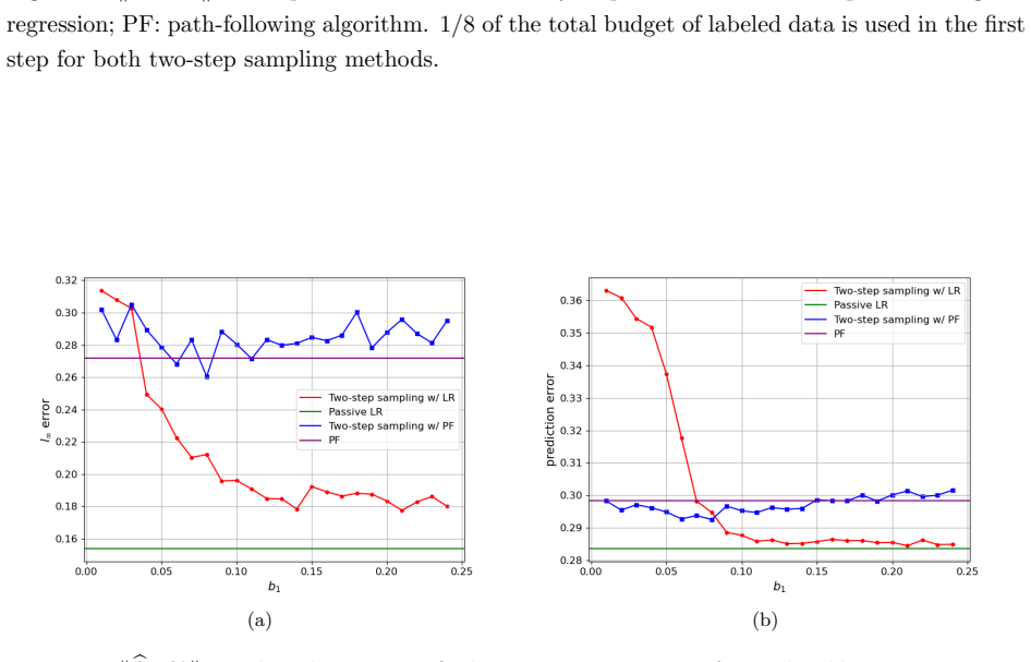
- [Section 5] The simulations set δ1 = δ2 = 1 and use a Gaussian kernel, whereas the theory (Theorems 2–4) assumes a compactly supported kernel of order l with bandwidths δ_k → 0 that are specific functions of s, d, N, and n. The text explains the practical choice, but it would be helpful to comment explicitly on the gap between the implemented bandwidth and the theoretical regime, and on whether the simulation results should be interpreted as supporting the theoretical rates or only the algorithm's practical performance.
Circularity Check
Rates are not fitted, but the appendix's verification of the load-bearing RSC/RSM assumption invokes Theorem 2's own rate conclusions, making that support circular.
-
self definitional
[Section A.7 (verification of Assumption 3.5), opening paragraph; Assumption 3.5 in Section 3.1]
"Recall that in Theorem 2, we showed that with high probability, ∥ bθ1 − θ∗∥2 ≲ (s log d/N)^{β/(2β+1)} and ∥ bθk − θ∗∥2 ≲ (s log d/N)^{1/2} for 2 ≤ k ≤ K. ... Therefore, it suffices to verify Assumption 3.5 on the set Ω = {θ : ∥θ − bθk−1∥2 ≲ (s log d/N)^{β/(2β+1)}} at the kth iteration for any 2 ≤ k ≤ K."
Assumption 3.5 is one of the assumptions under which Theorem 2 is proved (Theorems 2-4 are stated under Assumptions 3.1-3.5). The appendix's 'detailed verification' of Assumption 3.5 chooses the localized set Ω_{k-1} using the rates of bθ_{k-1} that are exactly the conclusions of Theorem 2 (for k≥2, the parametric rate; for k=2, the bθ1 rate from Theorem 1). Thus the RSC/RSM premise is justified by the same theorem that requires it. A simultaneous-induction reformulation could repair this, but as written the verification is not independent. Separately, Proposition A.4's condition (A.76) is incompatible with Theorem 2's δ_k ≍ (s log d/N)^{1/(2β)} tuning for β in ((1+√3)/2, (3+√15)/2), so the appendix does not establish the condition under the theorem's own tuning in that regime.
full rationale
The main rate derivation (Theorem 1 to Theorems 2-4) is not circular: the master rate comes from balancing kernel bias cn,kδ^β with stochastic error sqrt(cn,kK log d/(nδ_k)) via λ_k and δ_k, and the parametric rate follows algebraically from bk−1 = Δ^{1/(2β)} satisfying bk−1 ≥ Cδ_k and the event W_{k−1}; the phase-transition threshold (1+√3)/2 is the feasibility condition for that choice. The N-budget lower bound is an independent hypothesis-construction argument with θ_j at the target scale, not fitted to the upper bound. Self-citations to Feng et al. (2022) for path-following lemmas and the k=1 RSC base case are load-bearing but external published support, so they do not by themselves make the argument circular. The circularity I do find is localized to Section A.7: the paper says it verifies Assumption 3.5, but the verification uses Theorem 2's rate bounds, which are proved under Assumption 3.5. Because Assumption 3.5 is the load-bearing condition through which all upper-bound rates pass, this circular verification is material; the honest reading is that Theorems 2-4 are valid conditional implications, while the claimed verification of the condition for the conditional mean model is not self-contained. There is also a non-circular correctness gap: condition (A.76) fails under Theorem 2's tuning for a large part of the claimed β-range. Score 4 reflects a central claim with independent content and one partially circular support step, not a derivation that reduces to its inputs.
Assumptions & free parameters
free parameters (4)
- Active set half-width b_{k-1} =
c3(s log d/N)^(1/(2 beta)) in Theorem 2; cross-validated in Algorithm 3
- Bandwidth delta_k =
c1(s log d/N)^(1/(2 beta+1)) in the first step and b-dependent values later; set to 1 in simulations
- Regularization parameter lambda_k =
c2 sqrt(N log d/(n^2 b_{k-1} delta_k)); tuned by 5-fold CV in practice
- Smoothness parameter beta =
assumed known in all theorems; not estimated
assumptions (7)
- domain assumption Assumption 3.1: theta* is s-sparse with ||theta*||_0 <= s and ||theta*||_2 <= C.
- domain assumption Assumption 3.2: Z is bounded or sub-Gaussian, P(Y=1) is bounded away from 0 and 1, and sparse eigenvalues of E[ZZ^T | Y=y] are bounded.
- domain assumption Assumption 3.3: The conditional density f(x|y,z) is beta-Holder at x = theta*^T z with beta >= 1, with upper and lower bounds in a neighborhood of the threshold.
- standard math Assumption 3.4: The kernel K is of order l = floor(beta), symmetric, bounded, with finite moment conditions.
- ad hoc to paper Assumption 3.5: Restricted strong convexity and restricted smoothness of the subsampled smoothed risk on localized balls hold with constants proportional to the sampling probability.
- domain assumption Sample size conditions (3.11), (3.13), (3.19): the pool size n must be large relative to the budget N, e.g. N <= C n^(2 beta/(2 beta+1)) (s log d)^(1/(2 beta+1)).
- domain assumption For the lower bound, the sampling class Q_N(P(beta,s)) imposes conditional independence, budget E sum Q_i <= N, and a sparse eigenvalue bound on the sampled design.
Cite this review
Pith. "Pith review of Active Subsampling for Measurement-Constrained M-Estimation of Individualized Thresholds with High-Dimensional Data." pith.science (2026). https://pith.science/paper/OBPFCX3D
@misc{pith2026241113763,
  author       = {Pith},
  title        = {Pith review of: Active Subsampling for Measurement-Constrained M-Estimation of Individualized Thresholds with High-Dimensional Data},
  year         = {2026},
  howpublished = {\url{https://pith.science/paper/OBPFCX3D}},
  note         = {Machine review of arXiv:2411.13763}
}
abstract
Measurement-constrained problems frequently arise in modern applications such as electronic health record studies. In such problems, despite the availability of large datasets, collecting labeled data can be highly costly or time-consuming, allowing only a small portion of the data to be labeled within a given budget. This raises a critical question: which data points are most beneficial to label given the budget constraint? We study this question in the context of estimating an optimal individualized threshold under a measurement-constrained M-estimation framework. In particular, our goal is to estimate a high-dimensional parameter $\theta$ in a linear threshold $\theta^TZ$ for a continuous variable $X$ such that the discrepancy between whether $X$ exceeds the threshold $\theta^TZ$ and a binary outcome $Y$ is minimized. In the measurement-constrained setting, we propose a novel $K$-step active subsampling algorithm to estimate $\theta$, which iteratively samples the most informative observations in the dataset and solves a regularized M-estimator. Our theoretical analysis reveals a sharp phase transition phenomenon with respect to $\beta$, the smoothness of the conditional density of $X$ given $Y$ and $Z$. Please see the paper for the full abstract.
Figures


Figures from the paper (9 more)




Reference graph
Works this paper leans on
-
[1]
write newline
" write newline "" before.all 'output.state := FUNCTION format.url url empty "" url if FUNCTION article output.bibitem format.authors "author" output.check author format.key output output.year.check new.block format.title "title" output.check new.block crossref missing format.jour.vol output format.article.crossref output.nonnull format.pages output if ne...
-
[2]
Balcan, M.-F. , Broder, A. and Zhang, T. (2007). Margin based active learning. In International Conference on Computational Learning Theory. Springer
work page 2007
-
[3]
Balcan, M.-F. and Long, P. (2013). Active and passive learning of linear separators under log-concave distributions. In Conference on Learning Theory. PMLR
work page 2013
-
[4]
Baldwin, D. , Villanueva, G. , McNutt, R. and Bhatnagar, S. (2005). Eliminating inpatient sliding-scale insulin: a reeducation project with medical house staff. Diabetes care 28 1008--1011
work page 2005
-
[5]
and Van De Geer, S
B \"u hlmann, P. and Van De Geer, S. (2011). Statistics for high-dimensional data: methods, theory and applications. Springer Science & Business Media
2011
-
[6]
Castro, R. M. and Nowak, R. D. (2008). Minimax bounds for active learning. IEEE Transactions on Information Theory 54 2339--2353
work page 2008
- [7]
-
[8]
Clore, J. , Cios, K. , DeShazo, J. and Strack, B. (2014). Diabetes 130-US Hospitals for Years 1999-2008 . UCI Machine Learning Repository. DOI : https://doi.org/10.24432/C5230J
doi:10.24432/c5230j 2014
Show all 38 references
-
[9]
, Mahoney, M
Drineas, P. , Mahoney, M. W. , Muthukrishnan, S. and Sarl \'o s, T. (2011). Faster least squares approximation. Numerische mathematik 117 219--249
2011
-
[10]
, Duan, J
Feng, H. , Duan, J. , Ning, Y. and Zhao, J. (2024). Test of significance for high-dimensional thresholds with application to individualized minimal clinically important difference. Journal of the American Statistical Association 119 1396--1408
2024
-
[11]
, Ning, Y
Feng, H. , Ning, Y. and Zhao, J. (2022). Nonregular and minimax estimation of individualized thresholds in high dimension with binary responses. The Annals of Statistics 50 2284--2305
2022
-
[12]
and Hastie, T
Fithian, W. and Hastie, T. (2014). Local case-control sampling: Efficient subsampling in imbalanced data sets. Annals of statistics 42 1693
2014
-
[13]
, Hirshberg, D
Hadad, V. , Hirshberg, D. A. , Zhan, R. , Wager, S. and Athey, S. (2021). Confidence intervals for policy evaluation in adaptive experiments. Proceedings of the national academy of sciences 118 e2014602118
2021
-
[14]
, Hirano, K
Hahn, J. , Hirano, K. and Karlan, D. (2011). Adaptive experimental design using the propensity score. Journal of Business & Economic Statistics 29 96--108
2011
-
[15]
, Wang, J
Hedayat, A. , Wang, J. and Xu, T. (2015). Minimum clinically important difference in medical studies. Biometrics 71 33--41
2015
-
[16]
, Singer, J
Jaeschke, R. , Singer, J. and Guyatt, G. H. (1989). Measurement of health status: ascertaining the minimal clinically important difference. Controlled clinical trials 10 407--415
1989
-
[17]
and Pollard, D
Kim, J. and Pollard, D. (1990). Cube root asymptotics. The Annals of Statistics 191--219
1990
-
[18]
Koltchinskii, V. (2010). Rademacher complexities and bounding the excess risk in active learning. The Journal of Machine Learning Research 11 2457--2485
2010
-
[19]
, Mahoney, M
Ma, P. , Mahoney, M. and Yu, B. (2014). A statistical perspective on algorithmic leveraging. In International conference on machine learning. PMLR
2014
-
[20]
, Banerjee, M
Mallik, A. , Banerjee, M. and Michailidis, G. (2020). M-estimation in multistage sampling procedures. Sankhya A 82 261--309
2020
-
[21]
Manski, C. F. (1975). Maximum score estimation of the stochastic utility model of choice. Journal of econometrics 3 205--228
1975
-
[22]
, Banerjee, M
Mukherjee, D. , Banerjee, M. and Ritov, Y. (2021). Optimal linear discriminators for the discrete choice model in growing dimensions. The Annals of Statistics 49 3324--3357
2021
-
[23]
Nesterov, Y. (2013). Gradient methods for minimizing composite functions. Mathematical programming 140 125--161
2013
-
[24]
Perera, H. N. , Fahimnia, B. and Tokar, T. (2020). Inventory and ordering decisions: a systematic review on research driven through behavioral experiments. International Journal of Operations & Production Management 40 997--1039
2020
-
[25]
and Mahoney, M
Raskutti, G. and Mahoney, M. W. (2016). A statistical perspective on randomized sketching for ordinary least-squares. Journal of Machine Learning Research 17 1--31
2016
-
[26]
, DeShazo, J
Strack, B. , DeShazo, J. P. , Gennings, C. , Olmo, J. L. , Ventura, S. , Cios, K. J. and Clore, J. N. (2014). Impact of hba1c measurement on hospital readmission rates: Analysis of 70,000 clinical database patient records. BioMed Research International 2014 781670. ://onlineli...
2014 doi
-
[27]
Tsybakov, A. B. (2008). Introduction to Nonparametric Estimation. 1st ed. Springer Publishing Company, Incorporated
2008
-
[28]
, Yang, M
Wang, H. , Yang, M. and Stufken, J. (2019). Information-based optimal subdata selection for big data linear regression. Journal of the American Statistical Association 114 393--405
2019
-
[29]
, Zhu, R
Wang, H. , Zhu, R. and Ma, P. (2018). Optimal subsampling for large sample logistic regression. Journal of the American Statistical Association 113 829--844
2018
-
[30]
and Singh, A
Wang, Y. and Singh, A. (2016). Noise-adaptive margin-based active learning and lower bounds under tsybakov noise condition. In Thirtieth AAAI Conference on Artificial Intelligence
2016
-
[31]
Wang, Y. , Yu, A. W. and Singh, A. (2017). On computationally tractable selection of experiments in measurement-constrained regression models. Journal of Machine Learning Research 18 1--41
2017
-
[32]
, Wang, J
Xu, T. , Wang, J. and Fang, Y. (2014). A model-free estimation for the covariate-adjusted youden index and its associated cut-point. Statistics in Medicine 33 4963--4974. ://onlinelibrary.wiley.com/doi/abs/10.1002/sim.6290
2014 doi
-
[33]
, Ning, Y
Zhang, T. , Ning, Y. and Ruppert, D. (2021). Optimal sampling for generalized linear models under measurement constraints. Journal of Computational and Graphical Statistics 30 106--114
2021
-
[34]
, Zeng, D
Zhao, Y. , Zeng, D. , Rush, A. J. and Kosorok, M. R. (2012). Estimating individualized treatment rules using outcome weighted learning. Journal of the American Statistical Association 107 1106--1118
2012
-
[35]
, Zhao, J
Zhou, Z. , Zhao, J. and Bisson, L. J. (2020). Estimation of data adaptive minimal clinically important difference with a nonconvex optimization procedure. Statistical Methods in Medical Research 29 879--893
2020
-
[36]
and Cand \`e s, E
Zrnic, T. and Cand \`e s, E. J. (2024). Active statistical inference. arXiv preprint arXiv:2403.03208
2024 arXiv
-
[37]
, " * write output.state after.block = add.period write newline
ENTRY address author booktitle chapter edition editor howpublished institution journal key month note number organization pages publisher school series title type url volume year label extra.label sort.label short.list INTEGERS output.state before.all mid.sentence after.senten...
-
[38]
write newline
" write newline "" before.all 'output.state := FUNCTION n.dashify 't := "" t empty not t #1 #1 substring "-" = t #1 #2 substring "--" = not "--" * t #2 global.max substring 't := t #1 #1 substring "-" = "-" * t #2 global.max substring 't := while if t #1 #1 substring * t #2 gl...
Reviewed August 12, 2026 · model on record in the stance chip above.
Discussion (0). Continue with ORCID to comment.