REVIEW 4 major objections 4 minor 38 references
ICODE: Modeling Dynamical Systems with Extrinsic Input Information
T0 review · 4 major / 4 minor · reviewed 2026-08-12 · deepseek-v4-flash
Pith's one-line read Feeding external inputs directly into neural ODEs improves prediction on physical systems, with a contraction guarantee for fixed-point convergence.
desk verdict The empirical ICODE method is plausible and worth a look, but the advertised contraction-to-fixed-point theorem only proves incremental stability for time-varying inputs, so the central theoretical claim is false as stated. read the letter →
The pith
A machine-rendered reading of the paper's core claim, the machinery that carries it, and where it could break.
The reading
What carries the argument
The central object is the affine-in-input ICODE vector field $\dot{x} = \sum_i f_i(x) + \sum_j k_j(x)u_j$, in which the input $u$ multiplies state-dependent neural networks $k_j$. This is the input-concomitant coupling term; its role is to put the measured external input on the same footing as the state, so that the model does not have to infer $u$ from data or differentiate it in time. The contraction guarantee rests on the metric condition of Theorem 1: an invertible $L$ defining $M = L^\top L$, with the symmetrized pullback of the Jacobian bounded above by $-cI$; Corollary 1 gives the simpler sufficient condition that the largest eigenvalue of the symmetrized Jacobian of the whole vector field stays below $-c$.
What would settle it
Train ICODE and a standard NODE on a system where the true input enters nonlinearly, such as $\dot{x} = f(x) + g(x)u^2$ with $u$ switching piecewise, and compare prediction error on held-out input shapes; if ICODE loses its advantage while the paper's mechanism requires affine-in-$u$ structure, the central claim would be falsified. Alternatively, inspect a trained ICODE with trajectories observed not to converge despite the Corollary 1 condition holding, which would break the contraction guarantee.
Extended reading notes
Core claim
ICODEs are defined by $\dot{x} = f_0(x) + g(x)u$, where both $f_0$ and the columns of $g$ are neural networks, so the input enters the dynamics in the same multiplicative way that control inputs typically enter physical systems. The paper proves that if there is a uniformly positive definite metric $M = L^\top L$ such that the symmetrized generalized Jacobian $R$ satisfies $(R + R^\top)/2 \le -cI$, then the model is contracting: any two trajectories converge exponentially to each other, and the system converges to a fixed point independent of the initial condition. The experimental section argues that this structure, plus the absence of a derivative on $u$ (unlike neural CDEs), lets ICODE capture the coupling between state and input, giving consistently lower prediction errors than NODE, ANODE, and CDE, particularly when $u$ switches abruptly or is piecewise.
Load-bearing premise
The load-bearing premise is that the physical system is affine in the measured input $u$ and that $u$ is available accurately at every training and prediction time; if $u$ enters nonlinearly, is missing, or is heavily corrupted, the ICODE advantage can disappear.
Editorial extensions
If this is right
- If ICODE is right, then for systems that are affine in a measured input, a neural ODE can learn the state-input coupling directly, yielding accurate multi-step prediction even when the input switches at discontinuities within the test horizon.
- The contraction conditions give a training-independent stability certificate: under Theorem 1 or Corollary 1, predictions converge to the same fixed point from any initial condition, which is useful in safety-critical settings.
- Because the input enters as a multiplier rather than through a derivative, ICODE avoids the numerical amplification that piecewise inputs cause in neural CDEs, so performance holds as the input slope steepens.
- Scaling experiments indicate that ICODE benefits from larger width and depth, with training and validation loss both decreasing, suggesting the architecture is useful beyond small benchmark models.
- When the input span is zero or the input is independent of the state, ICODE reduces to standard NODE behavior, as the paper explicitly notes.
Reading between the lines
- The proof of Theorem 1 is not carried out in the paper; it is attributed to the contraction analysis in [27], so the convergence guarantee inherits the assumptions of that external contraction-analysis result.
- A natural next step the paper leaves open is to replace the affine-in-$u$ ansatz with a more general $\dot{x} = f(x,u)$, which the limitations section names as future work; one could test whether learned coupling terms can capture quadratic or logarithmic input dependencies.
- The contraction conditions are checkable during training; an implementation could monitor the spectral bound as a regularizer, a use not explored in the paper.
- The heat-conduction experiments suggest ICODE also serves for spatiotemporal PDEs when boundary or source terms are treated as inputs; a testable extension would be to compare against physics-informed baselines on the same PDE.
Editorial analysis
A structured set of objections, weighed in public.
Referee Report
Summary. The paper introduces Input Concomitant Neural ODEs (ICODEs), a neural-ODE architecture that is affine in the external input u, with separate subnetworks for the drift and input-coupling vector fields. The authors claim that a contraction condition, given in Theorem 1, guarantees that trajectories of the trained model converge to a fixed point regardless of initial conditions, and they support the method with prediction experiments on seven physical systems (single-link robot, DC-DC converter, rigid body, Rabinovich-Fabrikant equation, glycolytic-glycogenolytic pathway, swing equation, heat conduction), comparing against NODE, ANODE, and CDE variants, including noisy-input and scaling studies.
Significance. If the empirical claims are correct, ICODE is a useful and simple input-aware neural-ODE class, and the breadth of benchmarks plus the public code are assets. The core advertised theoretical contribution, however, is not supported: contraction of trajectories does not imply convergence to a fixed point when the input is time-varying, and condition (5) is never verified or enforced on trained models. The experimental comparison is also marred by internally inconsistent metric values (RMSE smaller than MAE in Tables I and VII), which casts doubt on the quantitative superiority claims as currently reported.
major comments (4)
- [Abstract and Section II (Theorem 1)] The central guarantee is stated as convergence to a fixed point, but Theorem 1 only establishes incremental stability. In Eq. (4), u(t) is a time-varying external signal, so the vector field is non-autonomous. Condition (5) gives exponential convergence of δy to 0, i.e., any two solutions converge to a common trajectory x*(t); it does not imply that x*(t) is constant. A concrete counterexample is ẋ = -x + sin(t), which has the ICODE form with f0(x) = -x, g(x) = 1, satisfies (5) with L = 1, yet every solution converges to a sinusoidal steady state rather than a fixed point. Thus the abstract's claim that 'system trajectories of the trained model converge to a fixed point, regardless of initial conditions' is false for the time-varying inputs used throughout the experiments. I ask the authors to either prove the fixed-point claim under an explicit extra assumption (e.g., u(t) → constant) or replace 'fixed point' with 'common trajectory' throughout the abstract, introduction, and conclusion.
- [Section II, condition (5) and Section III] Theorem 1 is not connected to the trained models: the paper never constructs the metric M(x), never checks whether condition (5) holds for any trained ICODE, and imposes no regularization or parameterization that would enforce contraction. The theorem is a restatement of the standard Lohmiller-Slotine criterion applied to the Jacobian of (4), and the proof explicitly defers to [27]. As a result, the statement in the introduction that 'theoretical guarantees are provided for the contraction property of ICODEs' overstates what is demonstrated. I request either (a) an algorithmic way to enforce or certify (5) on trained networks, with verification reported in the experiments, or (b) a clearly stated weakening of the contribution to 'a sufficient condition that holds for some ICODE instances, not verified here.'
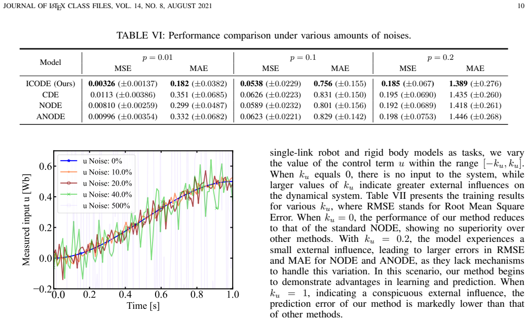
- [Tables I and VII] The reported RMSE values are smaller than the corresponding MAE values in several rows, which is impossible for any error sequence: RMSE ≥ MAE by Jensen's inequality. For example, Table I (single-link robot, Δu=0) reports RMSE = 0.027 and MAE = 0.065 for ICODE, and Table VII (single-link robot, ku=0) reports RMSE = 0.048 and MAE = 0.18. These entries strongly suggest that what is labeled 'RMSE' is actually mean squared error. If so, all quantitative comparisons in these tables need to be recomputed, re-labeled, or have their units clarified; the current reporting prevents the reader from assessing the claimed superior performance.
- [Section II, paragraph before Theorem 1] The text says contraction 'refers to the convergence of the models to the theoretical optimal solution throughout the learning process, despite variations in the initial conditions of the training processes.' This conflates two distinct notions: (i) trajectory convergence of a given dynamical system and (ii) convergence of the training algorithm to an optimal parameter set. Theorem 1 concerns only (i). This conflation is repeated in the 'Note to Practitioners' and in the contribution list, and it should be corrected to avoid implying that contraction of the learned vector field guarantees convergence of the training procedure.
minor comments (4)
- [Appendix A] The last sentence of Appendix A ends with the fragment 'significantly weaker.' after discussing ANODE's test-set performance; this should be completed or merged with the preceding sentence.
- [Section II, Eq. (3)] In Eq. (3), the activation functions are listed as h0, ..., h_{α−1}, s0, s_{β−1}, which omits s1 through s_{β−2}; the notation should be made consistent, such as s0, ..., s_{β−1}.
- [Figures 2, 4, 10] The units 'Wb' (weber) are used for control torque, switch signal, and other inputs; these quantities are not magnetic fluxes. The units should be corrected (e.g., N·m for torque in the robot example, dimensionless for the converter switch, etc.) or removed where the input is dimensionless.
- [Section III-A] The parameter 'q = 3.5 × 10^{-4}' is introduced without explanation; if this is a damping coefficient or other physical parameter, it should be named and its units given.
Circularity Check
No significant circularity: the contraction theorem is imported from an external criterion, the sole self-citation is peripheral, and the empirical claims are evaluated on held-out trajectories.
full rationale
The derivation chain is self-contained on the circularity axes that matter. Theorem 1's sufficient condition (Eq. 5) is the standard Lohmiller–Slotine contraction condition applied to the ICODE Jacobian J(x,u) = Σ∂f_i/∂x + Σ∂k_j/∂x u_j, and the paper explicitly attributes the proof methodology to [27]; no parameter fitted to the benchmark data is reused to define the contraction conclusion, so the theorem is not a renamed fit. The only self-citation with overlapping authorship is [33], used in the glycolytic-pathway experiment to motivate Transformer-integrated NODE variants; that citation is peripheral, and the experimental comparison does not rest on it. The benchmarks are generated from equations that are affine in u, matching Eq. (2), but the paper states this inductive-bias motivation explicitly and evaluates on held-out trajectories, so the empirical superiority claim is not a fitted quantity renamed as a prediction. A separate correctness gap, not a circularity, is that the abstract's 'converge to a fixed point' overstates Theorem 1: condition (5) proves δx(t)→0 between neighboring trajectories (as the proof itself stops at 'exponential convergence of δx to 0'), which for time-varying u means convergence to a common trajectory, not a constant equilibrium; the Limitations section likewise concerns input coupling, not this fixed-point issue. Since the circularity patterns are absent, the circularity score is 0.
Assumptions & free parameters
free parameters (2)
- Neural network weights for subnetworks f_i and k_j =
Learned on each benchmark via gradient descent (values not reported)
- Training hyperparameters (learning rate, network width, hidden layers, number of trajectories, ANODE augmentation) =
Table IX values, e.g., lr 5e-3 to 2e-3, width 50-200, layers 2-3
assumptions (4)
- standard math Lohmiller-Slotine contraction criterion (Theorem 1 and Corollary 1)
- domain assumption Target dynamics are affine in the external input u (Eq. (2))
- domain assumption External input u(t) is measured and available at training and inference time
- domain assumption Smoothness and invertibility of contraction metric L(x) and well-posedness of neural ODE initial value problems
Cite this review
Pith. "Pith review of ICODE: Modeling Dynamical Systems with Extrinsic Input Information." pith.science (2026). https://pith.science/paper/OATFFSPU
@misc{pith2026241113914,
  author       = {Pith},
  title        = {Pith review of: ICODE: Modeling Dynamical Systems with Extrinsic Input Information},
  year         = {2026},
  howpublished = {\url{https://pith.science/paper/OATFFSPU}},
  note         = {Machine review of arXiv:2411.13914}
}
read the original abstract
Learning models of dynamical systems with external inputs, which may be, for example, nonsmooth or piecewise, is crucial for studying complex phenomena and predicting future state evolution, which is essential for applications such as safety guarantees and decision-making. In this work, we introduce \emph{Input Concomitant Neural ODEs (ICODEs)}, which incorporate precise real-time input information into the learning process of the models, rather than treating the inputs as hidden parameters to be learned. The sufficient conditions to ensure the model's contraction property are provided to guarantee that system trajectories of the trained model converge to a fixed point, regardless of initial conditions across different training processes. We validate our method through experiments on several representative real dynamics: Single-link robot, DC-to-DC converter, motion dynamics of a rigid body, Rabinovich-Fabrikant equation, Glycolytic-glycogenolytic pathway model, and heat conduction equation. The experimental results demonstrate that our proposed ICODEs efficiently learn the ground truth systems, achieving superior prediction performance under both typical and atypical inputs. This work offers a valuable class of neural ODE models for understanding physical systems with explicit external input information, with potentially promising applications in fields such as physics and robotics. Our code is available online at https://github.com/EEE-ai59/ICODE.git.
Figures


Figures from the paper (9 more)




Reference graph
Works this paper leans on
-
[27]
On contraction analysis for non-linear systems,
W. Lohmiller and J.-J. E. Slotine, “On contraction analysis for non-linear systems,” Automatica, vol. 34, no. 6, pp. 683–696, 1998
1998
-
[1]
A. Roxin and A. Ledberg, “Neurobiological models of two-choice decision making can be reduced to a one-dimensional nonlinear diffusion equation,” PLoS Comput. Biol. , vol. 4, no. 3, p. e1000046, 2008
work page 2008
-
[2]
Dynamic decision making: Human control of complex systems,
B. Brehmer, “Dynamic decision making: Human control of complex systems,” Acta Psychol., vol. 81, no. 3, pp. 211–241, 1992
work page 1992
-
[3]
A scalable safety critical control framework for nonlinear systems,
T. Gurriet, M. Mote, A. Singletary, P. Nilsson, E. Feron, and A. D. Ames, “A scalable safety critical control framework for nonlinear systems,” IEEE Access, vol. 8, pp. 187 249–187 275, 2020
work page 2020
-
[4]
C. Sidrane, A. Maleki, A. Irfan, and M. J. Kochenderfer, “Overt: An algorithm for safety verification of neural network control policies for nonlinear systems,” J. Mach. Learn. Res. , vol. 23, no. 117, pp. 1–45, 2022
work page 2022
-
[5]
Neural ordinary differential equations,
R. T. Chen, Y . Rubanova, J. Bettencourt, and D. K. Duvenaud, “Neural ordinary differential equations,” Adv. Neural Inf. Process. Syst., vol. 31, 2018
work page 2018
-
[6]
E. Dupont, A. Doucet, and Y . W. Teh, “Augmented neural ODEs,” Adv. Neural Inf. Process. Syst. , vol. 32, 2019
work page 2019
-
[7]
Stable neural ODE with Lyapunov-stable equilibrium points for defending against adversarial attacks,
Q. Kang, Y . Song, Q. Ding, and W. P. Tay, “Stable neural ODE with Lyapunov-stable equilibrium points for defending against adversarial attacks,” Adv. Neural Inf. Process. Syst. , vol. 34, pp. 14 925–14 937, 2021
work page 2021
Show all 38 references
-
[8]
Stabilized neural differential equations for learning dynamics with explicit constraints,
A. White, N. Kilbertus, M. Gelbrecht, and N. Boers, “Stabilized neural differential equations for learning dynamics with explicit constraints,” Adv. Neural Inf. Process. Syst. , vol. 36, 2024
2024
-
[9]
Data-driven methods applied to soft robot modeling and control: A review,
Z. Chen, F. Renda, A. L. Gall, L. Mocellin, M. Bernabei, T. Dangel, G. Ciuti, M. Cianchetti, and C. Stefanini, “Data-driven methods applied to soft robot modeling and control: A review,” IEEE Trans. Autom. Sci. Eng., pp. 1–16, 2024
2024
-
[10]
Robust tracking control of heterogeneous robots with uncertainty: A super-exponential convergence neurodynamic approach,
D. Chen, L. Zhuo, Y . Shao, S. Li, C. Griffiths, and A. A. Fahmy, “Robust tracking control of heterogeneous robots with uncertainty: A super-exponential convergence neurodynamic approach,” IEEE Trans. Autom. Sci. Eng. , 2023
2023
-
[11]
Neural network stochastic differential equation models with applications to financial data forecast- ing,
L. Yang, T. Gao, Y . Lu, J. Duan, and T. Liu, “Neural network stochastic differential equation models with applications to financial data forecast- ing,” Appl. Math. Model. , vol. 115, pp. 279–299, 2023
2023
-
[12]
Towards neural earth system modelling by integrating artificial intelligence in earth system science,
C. Irrgang, N. Boers, M. Sonnewald, E. A. Barnes, C. Kadow, J. Staneva, and J. Saynisch-Wagner, “Towards neural earth system modelling by integrating artificial intelligence in earth system science,” Nat. Mach. Intell., vol. 3, no. 8, pp. 667–674, 2021
2021
-
[13]
Ankle joint torque estimation using an emg-driven neuromusculoskeletal model and an artificial neural network model,
L. Zhang, Z. Li, Y . Hu, C. Smith, E. M. G. Farewik, and R. Wang, “Ankle joint torque estimation using an emg-driven neuromusculoskeletal model and an artificial neural network model,” IEEE Trans. Autom. Sci. Eng. , vol. 18, no. 2, pp. 564–573, 2021
2021
-
[14]
Neural controlled differential equations for irregular time series,
P. Kidger, J. Morrill, J. Foster, and T. Lyons, “Neural controlled differential equations for irregular time series,” Adv. Neural Inf. Process. Syst., vol. 33, pp. 6696–6707, 2020
2020
-
[15]
Lyanet: A Lyapunov frame- work for training neural ODEs,
I. D. J. Rodriguez, A. Ames, and Y . Yue, “Lyanet: A Lyapunov frame- work for training neural ODEs,” in Int. Conf. Mach. Learn. PMLR, 2022, pp. 18 687–18 703
2022
-
[16]
Stable neural flows,
S. Massaroli, M. Poli, M. Bin, J. Park, A. Yamashita, and H. Asama, “Stable neural flows,” arXiv preprint arXiv:2003.08063 , 2020
2003 arXiv
-
[17]
Robust classification using contractive Hamiltonian neural ODEs,
M. Zakwan, L. Xu, and G. Ferrari-Trecate, “Robust classification using contractive Hamiltonian neural ODEs,” IEEE Control Syst. Lett. , vol. 7, pp. 145–150, 2022
2022
-
[18]
Learning stabilizable dynamical systems via control contraction metrics,
S. Singh, V . Sindhwani, J.-J. E. Slotine, and M. Pavone, “Learning stabilizable dynamical systems via control contraction metrics,” in Int. Work. Algorithm. Found. Robot.. Springer, 2018, pp. 179–195
2018
-
[19]
Vid- ode: Continuous-time video generation with neural ordinary differential equation,
S. Park, K. Kim, J. Lee, J. Choo, J. Lee, S. Kim, and E. Choi, “Vid- ode: Continuous-time video generation with neural ordinary differential equation,” in Proc. AAAI Conf. Artif. Intell. , vol. 35, no. 3, 2021, pp. 2412–2422
2021
-
[20]
Deep learning adapted to differential neural networks used as pattern classifi- cation of electrophysiological signals,
D. Llorente-Vidrio, M. Ballesteros, I. Salgado, and I. Chairez, “Deep learning adapted to differential neural networks used as pattern classifi- cation of electrophysiological signals,” IEEE Trans. Pattern Anal. Mach. Intell., vol. 44, no. 9, pp. 4807–4818, 2021
2021
-
[21]
Physics-informed neural networks for the shallow-water equations on the sphere,
A. Bihlo and R. O. Popovych, “Physics-informed neural networks for the shallow-water equations on the sphere,” J. Comput. Phys. , vol. 456, p. 111024, 2022
2022
-
[22]
Physics-informed neural networks: A deep learning framework for solving forward and inverse problems involving nonlinear partial differential equations,
M. Raissi, P. Perdikaris, and G. E. Karniadakis, “Physics-informed neural networks: A deep learning framework for solving forward and inverse problems involving nonlinear partial differential equations,” J. Comput. Phys., vol. 378, pp. 686–707, 2019
2019
-
[23]
Towards complex dy- namic physics system simulation with graph neural ordinary equations,
G. Shi, D. Zhang, M. Jin, S. Pan, and S. Y . Philip, “Towards complex dy- namic physics system simulation with graph neural ordinary equations,” Neural Netw., p. 106341, 2024
2024
-
[24]
Stochastic physics-informed neural ordinary differential equations,
J. O’Leary, J. A. Paulson, and A. Mesbah, “Stochastic physics-informed neural ordinary differential equations,” J. Comput. Phys. , vol. 468, p. 111466, 2022
2022
-
[25]
Hamiltonian neural net- works,
S. Greydanus, M. Dzamba, and J. Yosinski, “Hamiltonian neural net- works,” Adv. Neural Inf. Process. Syst. , vol. 32, 2019
2019
-
[26]
Lagrangian neural networks,
M. Cranmer, S. Greydanus, S. Hoyer, P. Battaglia, D. Spergel, and S. Ho, “Lagrangian neural networks,” arXiv preprint arXiv:2003.04630 , 2020
2003 arXiv
-
[28]
Rigid-body attitude control,
N. A. Chaturvedi, A. K. Sanyal, and N. H. McClamroch, “Rigid-body attitude control,” IEEE Control Syst. , vol. 31, no. 3, pp. 30–51, 2011
2011
-
[29]
Stochastic self-modulation of waves in nonequilibrium media,
M. I. Rabinovich and A. L. Fabrikant, “Stochastic self-modulation of waves in nonequilibrium media,” J. Exp. Theor. Phys., vol. 77, pp. 617– 629, 1979
1979
-
[30]
Modelization and experimental studies on the control of the glycolytic-glycogenolytic pathway in rat liver,
N. V . Torres, “Modelization and experimental studies on the control of the glycolytic-glycogenolytic pathway in rat liver,” Mol. Cell. Biochem., vol. 132, pp. 117–126, 1994
1994
-
[31]
Intervention in biological phenomena via feedback linearization,
M. A. Fnaiech, H. Nounou, M. Nounou, and A. Datta, “Intervention in biological phenomena via feedback linearization,” Adv. Bioinformatics., vol. 2012, no. 1, p. 534810, 2012
2012
-
[32]
A neural ODE interpretation of transformer layers,
Y . D. Zhong, T. Zhang, A. Chakraborty, and B. Dey, “A neural ODE interpretation of transformer layers,” in Symb. Deep Learn. Differ. Equ. II, 2022
2022
-
[33]
Controlsynth neural ODEs: Modeling dynamical systems with guaranteed convergence,
W. Mei, D. Zheng, and S. Li, “Controlsynth neural ODEs: Modeling dynamical systems with guaranteed convergence,” Adv. Neural Inf. Process. Syst., 2024
2024
-
[34]
Power system stability,
P. Kundur, “Power system stability,” Power system stability and control, vol. 10, no. 1, pp. 7–1, 2007
2007
-
[35]
On neural differential equations,
P. Kidger, “On neural differential equations,” arXiv preprint arXiv:2202.02435, 2022. JOURNAL OF LATEX CLASS FILES, VOL. 14, NO. 8, AUGUST 2021 13 APPENDIX A. A brief introduction of existing neural ODEs and their comparison with ICODE In this section, we briefly introduce the...
2022 arXiv
-
[36]
In many cases, fθ is implemented using a standard neural network architecture, such as a feedforward or convolutional network
Neural Ordinary Differential Equations: The Neural Ordinary Differential Equation (NODE or neural ODE) is defined as follows [5]: y(0) = y0, dy dt (t) = fθ(t, y(t)), (12) where y0 ∈ Rdy denotes the initial condition, θ is a vector of learnable parameters, and fθ : R × Rdy → Rd...
-
[37]
Neural Controlled Differential Equation: The Neural Controlled Differential Equation (CDE) enhances classical NODEs from a mathematical perspective, enabling the effec- tive processing of incoming data. The state of a neural ODE can be expressed in the form of the following Ri...
-
[38]
Augmented Neural ODE: The Augmented Neural Ordi- nary Differential Equation (ANODE) has been shown to learn representations that preserve the topology of the input space, resulting in certain functions that the NODE cannot represent. To address this limitation, ANODE [6] augme...
2021
Reviewed August 12, 2026 · model on record in the stance chip above.
Discussion (0). Continue with ORCID to comment.