Sample space filling analysis for boson sampling validation

A.A. Mazanik; A.N. Rubtsov

REVIEW 5 major objections 5 minor 40 references

Sample space filling analysis for boson sampling validation

T0 review · 5 major / 5 minor · reviewed 2026-08-12 · deepseek-v4-flash

Challenge this review Re-run · record.json Download PDF Read on arXiv ↗ Review JSON

Pith's one-line read A boson-sampling validator based on how samples fill the outcome space can distinguish genuine boson sampling from classically simulatable alternatives using only measured samples and pairwise distances, with no permanent computations.

desk verdict A simple, reproducible filling-curve fingerprint that separates boson sampling from distinguishable particles at scale, but the abstract overclaims against classical spoofers that the paper's own figure shows are not separated. read the letter →

arxiv 2411.14076 v1 pith:AR2JVDST submitted 2024-11-21 quant-ph

A.A. Mazanik , A.N. Rubtsov This is my paper · ORCID

classification quant-ph

keywords bosonsamplingvalidationprotocolwavefunctionnetworksamplespacefillingdistinguishableparticlesmean-fieldquantumadvantagedegreedistribution

verification ladder T0 review T1 audit T2 compute T3 formal

The pith

A machine-rendered reading of the paper's core claim, the machinery that carries it, and where it could break.

The reading

Boson-sampling experiments must convince skeptics that their outputs come from the true multi-photon distribution rather than from a classically simulatable substitute, and this paper proposes a cheap method for doing so. It builds a graph, called a wave function network, from the measured samples and tracks how the mean and spread of the sample degree distribution grow as more samples are collected. The paper claims these growth curves have a fixed low-order polynomial shape and that their fitted coefficients are fingerprints of the sampling mechanism. For a 5-photon, 25-mode circuit the fitted error ellipsoids for boson sampling, distinguishable-particle, and mean-field samplers do not overlap; for 7, 12, and 20 photons in 49, 144, and 400 modes, boson sampling separates from distinguishable particles on public data. If the claim is right, experimenters can validate large boson-sampling runs without computing permanents and without huge sample counts.

What carries the argument

The wave function network is a graph whose vertices are the collected samples $X_i$, with an edge between two samples when their L1 distance $d(X_i,X_j)=\sum_p |n^{(i)}_p-n^{(j)}_p|$ is below an activation radius $R$. The method measures the average degree $\mu$ and the standard deviation $\sigma$ of the degree distribution of this graph as the number of samples $N$ grows, fits the two growth curves with the polynomials of Eq. (4), and uses the fitted coefficients as the discriminating features. The practical load is just the pairwise distance computation between samples, with no permanents and no trained classifier; this is why the method can be applied at 20 photons in 400 modes.

What would settle it

Take the n=7, m=49 setup and sweep the activation radius R from just above 0 to large values; if the boson-sampling and distinguishable-particle clusters in the $(\alpha_\mu,\beta_\sigma)$ plane overlap for any R other than the manually chosen 8, or if $\alpha_\sigma$ becomes nonzero when the sample count is extended beyond 18,000, the intrinsic-fingerprint claim fails.

Watch

Extended reading notes

Core claim

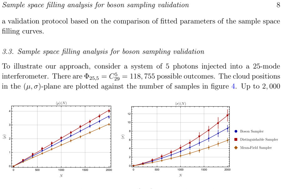
The central claim is that the filling of sample space by boson-sampling outputs carries an intrinsic signature of the wave function, visible in the growth of a network built from samples. With the L1 metric and a fixed activation distance $R$, the mean degree of the network grows as $\langle\mu\rangle(N)=\alpha_\mu N$, and the standard deviation of the degree grows as $\langle\sigma\rangle(N)=\alpha_\sigma N+\beta_\sigma N^2$ over the sample numbers available in practice. The coefficients $\alpha_\mu,\alpha_\sigma,\beta_\sigma$ are proposed as snapshot-count-independent fingerprints of the sampler inside the black box. The paper shows that for $n=5,m=25$ these coefficients form non-overlapping error ellipsoids separating boson sampling from distinguishable-particle and mean-field sampling, both for a fixed unitary and when averaged over unitaries; the uniform case is noted as trivially excluded by single-particle observables. Using the data in [40], it further shows that with two surviving coefficients $\alpha_\mu$ and $\beta_\sigma$, boson sampling separates from distinguishable particles for $n=7,12,20$ photons in $m=49,144,400$ modes, within a collision-free subspace. The authors conclude that the approach is an efficient, permanent-free validation protocol for current and near-term experiments.

Load-bearing premise

The method's separation depends on the asserted polynomial forms in Eq. (4), with coefficients that are stable across sample count N, activation radius R, and interferometer realization; if any of these stabilities breaks, the distinguishable error ellipsoids may reflect analysis choices rather than an intrinsic property of the sampler.

Editorial extensions

If this is right

The protocol can reject distinguishable-particle and mean-field hypotheses without evaluating permanents, making it a practical pre-screening test for experimental data.
Because it uses fitted coefficients rather than raw cloud positions, validation does not require matching the exact number of collected samples between different black boxes.
The method remains usable when data are restricted to a collision-free subspace, which is a harder case for validation and the natural regime for large photonic experiments.
Results on 20 photons in 400 modes suggest the test can be applied at sizes where direct distribution verification is impossible.

Reading between the lines

Editorial extensions of the paper, not claims the author makes directly.

A natural next test, not reported in the paper, is to measure the same coefficients on Gaussian boson sampling data, where the same network construction applies and a fingerprint might generalize.
The method's reliance on a manually chosen $R$ could be replaced by an automatic rule that picks $R$ to maximize the separation between the fitted ellipsoids; that would make the protocol parameter-free and testable on unknown black boxes.
Because the coefficients are fitted from growth curves, one could look for scale-invariant combinations such as $\beta_\sigma/\alpha_\mu^2$ that might transfer across system sizes, giving experimenters a calibrated decision threshold rather than relative cluster separation.

Share X Bluesky LinkedIn Reddit HN

Editorial analysis

A structured set of objections, weighed in public.

Desk editor's note, referee report, and a circularity audit.

Desk Editor's Note

read the letter

Short version: the paper has a genuinely simple idea — characterize samplers by the fitted slope and curvature of the WFN degree statistics as a function of sample count — and it demonstrates that the resulting fingerprint separates ideal boson sampling from distinguishable-particle sampling at up to n=20, m=400, using public data from Neville et al. That is a real, reproducible result, and the authors deserve credit for shipping code and being transparent about which data they used.

The trouble is the abstract. It says the filling behavior can be 'efficiently distinguished from classically simulated cases,' but the scale tests only separate boson sampling from distinguishable particles. The same Bristol data contain a rejection sampler and two Monte-Carlo samplers — exactly the kind of classical spoofers a validation protocol should reject — and Figure 6 shows those sit essentially on top of the boson sampling cluster. The authors acknowledge this in the Discussion, so the gap is not hidden, but the headline claim and the validation protocol as stated are broader than the demonstrated evidence. The mean-field sampler, the hardest mock-up, also disappears after n=5, so we don't know how the fingerprint behaves against it at scale.

There are two further soft spots that are real but more minor. Equation (4) is an empirical ansatz: we get no derivation or error analysis for the polynomial form, and the paper's own n>=7 results show the quadratic term vanishes, so the fingerprint itself changes form with system size. The activation radius R is tuned manually, and there is no sensitivity analysis, so the separation we see is at a selected operating point. Finally, the no-repetition assumption in Section 3.1 is problematic at n=5, m=25: with ~2,000 samples and only ~1.2e5 outcomes, collisions are near-certain, so either the data were filtered (which would bias the filling curve) or the assumption is silently violated.

None of this undermines the core observation. The filling-curve fingerprint is plausible and the clean separation against distinguishable particles is worth knowing about. But as it stands, the paper promises something the data don't show. A revised version that narrows the abstract, adds a sensitivity analysis for R, tests the mean-field sampler at scale, and addresses the repeated-samples policy would be a solid contribution. I'd send it to review, with clear instructions to focus on those points.

Referee Report

5 major / 5 minor

Summary. The paper proposes a new boson sampling validation protocol based on the sample-space filling behavior of wave-function networks. For a set of N samples, the authors construct a graph with edges activated when the L1 distance between two samples is below a radius R, then examine the mean μ and standard deviation σ of the degree distribution as functions of N. They assert that in the accessible regime the filling curves obey μ = α_μ N and σ = α_σ N + β_σ N^2 (Eq. 4), and that the fitted coefficients (α_μ, α_σ, β_σ) are intrinsic fingerprints of the sampling procedure. The protocol is demonstrated at n=5, m=25 for boson sampling, distinguishable-particle sampling, and mean-field sampling, with error ellipsoids reported as non-overlapping. Using the Bristol dataset of Ref. [40], the authors test the protocol for n=7, 12, and 20 photons in 49-, 144-, and 400-mode interferometers, reporting separation between ideal boson sampling and distinguishable-particle sampling. The abstract claims that boson sampling filling behavior 'can be computationally efficiently distinguished from classically simulated cases.'

Significance. If the central claim holds, the approach would provide a simple, permanent-free, sample-efficient validation tool that can complement existing protocols for photonic boson sampling experiments. The paper's strengths include the use of publicly available experimental data from [40], open-source code, and a concrete demonstration that a network-based statistic separates distinguishable-particle sampling from boson sampling at moderately large scales (up to n=20, m=400). The method's computational cost is stated to be dominated by pairwise distances, with potential improvements via nearest-neighbor search. The significance is conditional, however, because the demonstrated separation does not cover the full range of classical mock-up distributions claimed in the abstract, and because the fitted polynomial form and the manual choice of R are not yet backed by a derivation or a sensitivity analysis.

major comments (5)

[Abstract and Section 4, Figure 6] The abstract's claim that the filling behavior can be 'distinguished from classically simulated cases' is broader than the demonstrated evidence. In Figure 6, the only clear separation shown for n=7, 12, 20 is between ideal boson sampling and distinguishable-particle sampling; the rejection sampler and the two Monte-Carlo samplers are explicitly described in Section 4 as 'still much closer to the real boson sampling than to a set-up with distinguishable particles.' These samplers are exactly the classically simulated spoofers that a validation protocol should reject. The Discussion narrows the claim to distinguishable-particle sampling, but the abstract and the protocol description do not. Please either narrow the central claim to match the evidence or extend the experimental tests to show that the protocol can reject approximate classical samplers.
[Section 3.3, Eq. (4) and Table 1] The low-order polynomial form (4) is asserted without derivation or justification. The claim that α_μ, α_σ, and β_σ are intrinsic to the sampling procedure and independent of N is load-bearing, but the paper's own results show that the form is not stable: in Section 4, for n≥7, α_σ vanishes within errors, so the fitted model reduces from three parameters to two. The coefficients are also fit to the same kind of data that they classify, and the errors grow substantially when averaging over different unitaries (Figure 5b). A theoretical derivation of (4), or at minimum a systematic stability analysis over fit windows, R, and unitary ensembles, is needed to support the claim that these coefficients are intrinsic fingerprints rather than artifacts of the fitting procedure.
[Section 3.1, no-repetition assumption] The assumption that the sample set contains no repetitions (Xi≠Xj for all i≠j) is inconsistent with the n=5, m=25 demonstration. The sample space size is C(29,5)=118,755, and up to 2,000 samples are drawn. Under sampling with replacement, the probability of no collision is extremely small (approximately exp(-2000^2/(2·118755)) ≈ 10^-8). If the data were post-processed to remove repetitions, or if the samples were generated without replacement, this must be stated, and the impact on the filling curves and on the fitted parameters must be analyzed. If repetitions are instead neglected in the analysis, the approximation error needs to be quantified.
[Section 3.1 and Figure 6 caption] The activation radius R is described as an adjustable parameter that 'should be optimised to get the best result,' and the caption of Figure 6 states that R was 'optimised manually.' The reported separation is therefore shown only at a manually tuned operating point, with no sensitivity analysis. Since R directly controls the degree distribution and hence the fitted coefficients, the protocol's robustness to the choice of R (and to the fit window) must be demonstrated. Without such an analysis, the non-overlap of error ellipsoids in Figures 5 and 6 could reflect the tuning procedure rather than an intrinsic property of the sampling distributions.
[Section 4] The mean-field sampler, which the paper itself identifies as the most stringent classical mock-up distribution (Section 2.2), is tested only at n=5, m=25 and is absent from the larger n=7, 12, 20 tests. The paper notes that [40] contains no mean-field data, but this leaves open the question of whether the protocol scales to the hardest classical case. Please either include mean-field data at larger sizes, or clearly state the absence as a limitation of the current evidence and temper the protocol's claimed applicability.

minor comments (5)

[Section 3.2, Figure 3] Figure 3 shows dependence of cloud position on N, but the caption does not identify which curves correspond to which sampling procedure. Please add a legend or describe the line styles and colors in the caption.
[Section 3.3, Table 1] The error bars in Table 1 are reported for each fitted coefficient, but the number of sampling iterations and the number of unitary realizations used for the 'single U' and 'diff U' cases are not stated. Please provide these details, as they are needed to interpret the error ellipsoids in Figure 5.
[Section 3.3, Eq. (4)] The text says that the coefficients 'do not depend on the number of samples received by the validation program,' but the coefficients are themselves obtained by fitting over a range of N. Please clarify that this means the coefficients are asymptotically independent of the final sample count in the fitted regime, and specify the range of N used for the fits in each case.
[Section 4] The transition from three fitted parameters (α_μ, α_σ, β_σ) at n=5 to two parameters (α_μ, β_σ) at n≥7 is stated but not explained. A brief comment on why α_σ vanishes for larger systems would help the reader understand whether this is a physical effect or an artifact of the fit.
[Section 3.1] The phrase 'permanent-free' is used in the introduction and discussion, but the main text says 'does not involve the calculation of permanents' (Section 3.3). For consistency, use the same term throughout, and define it at first use.

Circularity Check

0 steps flagged · score 0.0 of 10

No significant circularity: the protocol is an empirical fitting and classification scheme, not a claim that derives a prediction from its fitted inputs.

full rationale

The paper's derivation chain does not contain a step in which a predicted outcome is equivalent, by construction, to a fitted input. Section 3.3 defines the network cloud positions (mu, sigma) as functions of the number of samples N and fits them to the low-order polynomials of Eq. (4); the fitted coefficients alpha_mu, alpha_sigma, beta_sigma are then used as descriptive fingerprints for the different samplers. This is an empirical validation procedure rather than a first-principles prediction: the paper does not claim that the separation is derived from the coefficients themselves, and the fitted quantities are not renamed as predictions. The demonstrations in Figs. 5 and 6 compare these fitted fingerprints across samplers on the same data, which is a legitimate, if potentially overfitting-prone, calibration exercise rather than circular reasoning. The external citations ([35], [36], [40]) are methodology and dataset sources, not self-citations carrying the argument. The no-repetition assumption, the manual optimization of the activation radius R, and the gap between the broad abstract claim about distinguishing 'classically simulated cases' and the evidence that mainly separates boson sampling from distinguishable-particle sampling are correctness and evidence limitations, not instances of definitional circularity. No specific equation can be exhibited where the claim reduces to its own input by construction.

Assumptions & free parameters 3 free parameters · 6 assumptions · 0 invented entities

The protocol introduces no new physical entities, but it rests on several unproved modeling choices: the polynomial filling-curve form, the manually tuned activation radius, the no-repetition idealization, and the fidelity of the external [40] datasets. The free parameters are the activation radii, the fitting windows, and the fitted fingerprint coefficients that carry the entire discrimination claim.

free parameters (3)

Activation radius R = 8, 18, 36 for n=7/12/20 systems; value for the n=5 system not stated
Manually optimized to give the best separation of sampler clouds; the protocol's success is only shown at the tuned values, with no robustness analysis (Fig. 6 caption, Section 3.1).
Fit window (number of samples included in the filling-curve fits) = up to 2,000 samples for n=5; up to 18,000 samples for n>=7
The polynomial form (4) is assumed valid only in the 'initial region' of the filling curves; where this region ends is chosen post hoc, and the claimed N-independence of the coefficients holds only within it.
Polynomial coefficients a_mu, a_sigma, b_sigma = Table 1 and Fig. 6 values, e.g., a_mu ~ 1.80e-3 for the n=5 boson sampler
These least-squares coefficients are the protocol's fingerprints, fitted to sample data; the central discrimination claim is entirely carried by them.

assumptions (6)

ad hoc to paper L1 metric with hard threshold d < R activates an edge between two samples
Section 3.1: the metric and activation rule are modeling choices, not derived from the boson sampling statistics.
ad hoc to paper Filling curves obey <mu> = a_mu N and <sigma> = a_sigma N + b_sigma N^2 in the accessible regime
Section 3.3: asserted from n=5 visual inspection; no derivation; the paper itself reports a_sigma to zero at n>=7, so the form is not universal.
ad hoc to paper Samples contain no repetitions (Xi != Xj)
Section 3.1: real boson sampling draws with replacement; at n=5, m=25 with N=2,000 over 118,755 outcomes, repetitions are essentially certain, and the protocol does not specify how to handle them.
domain assumption Input is n single photons in the first n modes of an m=n^2-mode interferometer with Haar-random unitary
Sections 2.1, 3.1: the protocol is demonstrated only in this standard setting.
domain assumption The [40] datasets faithfully represent the nominal samplers (boson, distinguishable, rejection, MCMC, brute-force)
Section 4: all large-scale conclusions rest on the correctness of the externally published Bristol data.
domain assumption Collision-free output subspace is the relevant test regime
Section 4: the large-scale data are restricted to at most one photon per mode; generalization to the collisional regime is untested.

how reviews work

0 comments

Cite this review

Pith. "Pith review of Sample space filling analysis for boson sampling validation." pith.science (2026). https://pith.science/paper/AR2JVDST

@misc{pith2026241114076,
  author       = {Pith},
  title        = {Pith review of: Sample space filling analysis for boson sampling validation},
  year         = {2026},
  howpublished = {\url{https://pith.science/paper/AR2JVDST}},
  note         = {Machine review of arXiv:2411.14076}
}

abstract

Achieving a quantum computational advantage regime, and thus providing evidence against the extended Church-Turing thesis, remains one of the key challenges of modern science. Boson sampling seems to be a very promising platform in this regard, but to be confident of attaining the advantage regime, one must provide evidence of operating with a correct boson sampling distribution, rather than with a pathological classically simulatable one. This problem is often called the validation problem, and it poses a major challenge to demonstrating unambiguous quantum advantage. In this work, using the recently proposed wave function network approach, we study the sample space filling behavior with increasing the number of collected samples. We show that due to the intrinsic nature of the boson sampling wave function, its filling behavior can be computationally efficiently distinguished from classically simulated cases. Therefore, we propose a new validation protocol based on the sample space filling analysis and test it for problems of up to $20$ photons injected into a $400$-mode interferometer. Due to its simplicity and computational efficiency, it can be used among other protocols to validate future experiments to provide more convincing results.

Figures

Figures reproduced from arXiv: 2411.14076 by the authors.

**Figure 1.** Boson sampling scheme. Single photon sources generate an initial Fock state, which is injected into an m-mode interferometer. It performs some unitary transformation on this input state, after which the output state is measured by single photon detectors. The red color schematically shows the detectors that have triggered. Since its initial proposal, many boson sampling experiments [9–16] have been carried out. To r… view at source ↗

**Figure 2.** Schematic representation of the boson sampling validation protocol. Some unknown black-box sampling device produces samples that are fed to the input of some validation program. This validation program must provide a convincing conclusion about the similarity of the received data to several mock-up distributions. observables reflecting certain properties of the interferometer to exclude a uniform distribution. More … view at source ↗

**Figure 3.** Dependence of the position of clouds in the plane (µ, σ) on the number of samples considered N for several sampling cases. The left image corresponds to the µcoordinate of the cloud, and the right one corresponds to the σ-coordinate. The vertical bars represent the variance of the distribution of cloud points along the corresponding axis and thus indicate the size of the cloud along this axis. However, for systems … view at source ↗

Figures from the paper (3 more)

**Figure 4.** Figure 4: Cloud position in the (µ, σ)-plane as a function of the number of collected samples up to 2, 000. The system size is n = 5, m = 25 with a fixed unitary transformation Uˆ. The vertical bars indicate the cloud size, and the solid lines represent the fitted curves (see (4…

**Figure 5.** Figure 5: Three fitted parameters of cloud position dependence on the number of collected samples, together with ellipsoids corresponding to their errors: (a) averaged over sampling iterations with a fixed interferometer, (b) averaged over sampling iterations with several differ…

**Figure 6.** Figure 6: Two fitted parameters αµ and βσ of cloud position dependence on the number of collected samples together with their errors. Up to 18, 000 samples considered; the activation distances R were optimised manually. (a): System size n = 7, m = 49; R = 8. (b): System size n =…

Discussion (0). Continue with ORCID to comment.

Reference graph

Works this paper leans on

40 extracted references · 39 canonical work pages

[40]

Neville A, Sparrow C, Clifford R, Johnston E, Birchall P M, Montanaro A and Laing A 2017 Nature Physics 13 1153–1157

work page 2017
[1]

Nielsen M A and Chuang I L 2010 Quantum Computation and Quantum Information(Cambridge university press)

work page 2010
[2]

Kaye P, Laflamme R and Mosca M 2006 An Introduction to Quantum Computing(OUP Oxford)

work page 2006
[3]

Comput.26 1484–1509 Sample space filling analysis for boson sampling validation 13

Shor P W 1997 SIAM J. Comput.26 1484–1509 Sample space filling analysis for boson sampling validation 13

work page 1997
[4]

Arute F, Arya K, Babbush R, Bacon D, Bardin J C, Barends R, Biswas R, Boixo S, Brandao F G S L, Buell D A, Burkett B, Chen Y, Chen Z, Chiaro B, Collins R, Courtney W, Dunsworth A, Farhi E, Foxen B, Fowler A, Gidney C, Giustina M, Graff R, Guerin K, Habegger S, Harrigan M P, Hartmann M J, Ho A, Hoffmann M, Huang T, Humble T S, Isakov S V, Jeffrey E, Jiang ...

work page 2019
[5]

Madsen L S, Laudenbach F, Askarani M F, Rortais F, Vincent T, Bulmer J F, Miatto F M, Neuhaus L, Helt L G and Collins M J 2022 Nature 606 75–81

work page 2022
[6]

Aaronson S and Arkhipov A 2011 The computational complexity of linear optics Proceedings of the Forty-Third Annual ACM Symposium on Theory of Computing(San Jose California USA: ACM) pp 333–342

work page 2011
[7]

Gard B T, Motes K R, Olson J P, Rohde P P and Dowling J P 2015 An Introduction to Boson- Sampling (WORLD SCIENTIFIC) pp 167–192

work page 2015

Show all 40 references

[8]

Brod D J, Galv˜ ao E F, Crespi A, Osellame R, Spagnolo N and Sciarrino F 2019Advanced Photonics 1 034001–034001
[9]

Crespi A, Osellame R, Ramponi R, Brod D J, Galvao E F, Spagnolo N, Vitelli C, Maiorino E, Mataloni P and Sciarrino F 2013 Nature photonics 7 545–549

2013
[10]

Tillmann M, Daki´ c B, Heilmann R, Nolte S, Szameit A and Walther P 2013 Nature photonics 7 540–544

2013
[11]

Spring J B, Metcalf B J, Humphreys P C, Kolthammer W S, Jin X M, Barbieri M, Datta A, Thomas-Peter N, Langford N K, Kundys D, Gates J C, Smith B J, Smith P G R and Walmsley I A 2013 Science 339 798–801

2013
[12]

Broome M A, Fedrizzi A, Rahimi-Keshari S, Dove J, Aaronson S, Ralph T C and White A G 2013 Science 339 794–798

2013
[13]

Wang H, He Y, Li Y H, Su Z E, Li B, Huang H L, Ding X, Chen M C, Liu C and Qin J 2017 Nature Photonics 11 361–365

2017
[14]

Loredo J C, Broome M A, Hilaire P, Gazzano O, Sagnes I, Lemaitre A, Almeida M P, Senellart P and White A G 2017 Phys. Rev. Lett.118 130503

2017
[15]

He Y, Ding X, Su Z E, Huang H L, Qin J, Wang C, Unsleber S, Chen C, Wang H, He Y M, Wang X L, Zhang W J, Chen S J, Schneider C, Kamp M, You L X, Wang Z, H¨ ofling S, Lu C Y and Pan J W 2017 Phys. Rev. Lett.118 190501

2017
[16]

Wang H, Li W, Jiang X, He Y M, Li Y H, Ding X, Chen M C, Qin J, Peng C Z, Schneider C, Kamp M, Zhang W J, Li H, You L X, Wang Z, Dowling J P, H¨ ofling S, Lu C Y and Pan J W 2018 Phys. Rev. Lett.120 230502

2018
[17]

Lund A P, Laing A, Rahimi-Keshari S, Rudolph T, O’Brien J L and Ralph T C 2014 Phys. Rev. Lett. 113 100502

2014
[18]

Hamilton C S, Kruse R, Sansoni L, Barkhofen S, Silberhorn C and Jex I 2017 Phys. Rev. Lett. 119 170501

2017
[19]

Adv.1 e1400255

Bentivegna M, Spagnolo N, Vitelli C, Flamini F, Viggianiello N, Latmiral L, Mataloni P, Brod D J, Galv˜ ao E F, Crespi A, Ramponi R, Osellame R and Sciarrino F 2015Sci. Adv.1 e1400255
[20]

Zhong H S, Li Y, Li W, Peng L C, Su Z E, Hu Y, He Y M, Ding X, Zhang W, Li H, Zhang L, Wang Z, You L, Wang X L, Jiang X, Li L, Chen Y A, Liu N L, Lu C Y and Pan J W 2018 Phys. Rev. Lett.121 250505

2018
[21]

Paesani S, Ding Y, Santagati R, Chakhmakhchyan L, Vigliar C, Rottwitt K, Oxenløwe L K, Wang J, Thompson M G and Laing A 2019 Nature Physics 15 925–929

2019
[22]

Zhong H S, Wang H, Deng Y H, Chen M C, Peng L C, Luo Y H, Qin J, Wu D, Ding X, Hu Y, Hu P, Yang X Y, Zhang W J, Li H, Li Y, Jiang X, Gan L, Yang G, You L, Wang Z, Li L, Liu Sample space filling analysis for boson sampling validation 14 N L, Lu C Y and Pan J W 2020 Science 370 ...

2020
[23]

Comput.14 1383–1423

Aaronson S and Arkhipov A 2014 Quantum Inf. Comput.14 1383–1423

2014
[24]

Carolan J, Meinecke J D, Shadbolt P J, Russell N J, Ismail N, W¨ orhoff K, Rudolph T, Thompson M G, O’brien J L and Matthews J C 2014 Nature Photonics 8 621–626

2014
[25]

Spagnolo N, Vitelli C, Bentivegna M, Brod D J, Crespi A, Flamini F, Giacomini S, Milani G, Ramponi R and Mataloni P 2014 Nature Photonics 8 615–620

2014
[26]

Liu K, Lund A P, Gu Y J and Ralph T C 2016 JOSA B 33 1835–1841

2016
[27]

Shchesnovich V S 2016 Phys. Rev. Lett.116 123601

2016
[28]

Walschaers M, Kuipers J, Urbina J D, Mayer K, Tichy M C, Richter K and Buchleitner A 2016 New Journal of Physics18 032001

2016
[29]

Giordani T, Flamini F, Pompili M, Viggianiello N, Spagnolo N, Crespi A, Osellame R, Wiebe N, Walschaers M and Buchleitner A 2018 Nature Photonics 12 173–178

2018
[30]

Viggianiello N, Flamini F, Innocenti L, Cozzolino D, Bentivegna M, Spagnolo N, Crespi A, Brod D J, Galv˜ ao E F and Osellame R 2018New Journal of Physics20 033017
[31]

Agresti I, Viggianiello N, Flamini F, Spagnolo N, Crespi A, Osellame R, Wiebe N and Sciarrino F 2019 Phys. Rev. X9 011013

2019
[32]

Flamini F, Walschaers M, Spagnolo N, Wiebe N, Buchleitner A and Sciarrino F 2020 Quantum Science and Technology5 045005

2020
[33]

Chabaud U, Grosshans F, Kashefi E and Markham D 2021 Quantum 5 578

2021
[34]

Giordani T, Mannucci V, Spagnolo N, Fumero M, Rampini A, Rodola E and Sciarrino F 2022 Quantum Science and Technology8 015005

2022
[35]

Iakovlev I A, Sotnikov O M, Dyakonov I V, Kiktenko E O, Fedorov A K, Straupe S S and Mazurenko V V 2023 Phys. Rev. A108 062420

2023
[36]

Mendes-Santos T, Schmitt M, Angelone A, Rodriguez A, Scholl P, Williams H J, Barredo D, Lahaye T, Browaeys A, Heyl M and Dalmonte M 2024 Phys. Rev. X14 021029

2024
[37]

Scheel S 2004 Permanents in linear optical networks ( Preprint quant-ph/0406127)

2004 arXiv
[38]

Tichy M C, Mayer K, Buchleitner A and Mølmer K 2014 Phys. Rev. Lett.113 020502

2014
[39]

Gogolin C, Kliesch M, Aolita L and Eisert J 2013 Boson-Sampling in the light of sample complexity (Preprint 1306.3995)

2013 arXiv

Pith tools

Reviewed August 12, 2026 · model on record in the stance chip above.

[1] [40]

Neville A, Sparrow C, Clifford R, Johnston E, Birchall P M, Montanaro A and Laing A 2017 Nature Physics 13 1153–1157

work page 2017

[2] [1]

Nielsen M A and Chuang I L 2010 Quantum Computation and Quantum Information(Cambridge university press)

work page 2010

[3] [2]

Kaye P, Laflamme R and Mosca M 2006 An Introduction to Quantum Computing(OUP Oxford)

work page 2006

[4] [3]

Comput.26 1484–1509 Sample space filling analysis for boson sampling validation 13

Shor P W 1997 SIAM J. Comput.26 1484–1509 Sample space filling analysis for boson sampling validation 13

work page 1997

[5] [4]

Arute F, Arya K, Babbush R, Bacon D, Bardin J C, Barends R, Biswas R, Boixo S, Brandao F G S L, Buell D A, Burkett B, Chen Y, Chen Z, Chiaro B, Collins R, Courtney W, Dunsworth A, Farhi E, Foxen B, Fowler A, Gidney C, Giustina M, Graff R, Guerin K, Habegger S, Harrigan M P, Hartmann M J, Ho A, Hoffmann M, Huang T, Humble T S, Isakov S V, Jeffrey E, Jiang ...

work page 2019

[6] [5]

Madsen L S, Laudenbach F, Askarani M F, Rortais F, Vincent T, Bulmer J F, Miatto F M, Neuhaus L, Helt L G and Collins M J 2022 Nature 606 75–81

work page 2022

[7] [6]

Aaronson S and Arkhipov A 2011 The computational complexity of linear optics Proceedings of the Forty-Third Annual ACM Symposium on Theory of Computing(San Jose California USA: ACM) pp 333–342

work page 2011

[8] [7]

Gard B T, Motes K R, Olson J P, Rohde P P and Dowling J P 2015 An Introduction to Boson- Sampling (WORLD SCIENTIFIC) pp 167–192

work page 2015