REVIEW 2 major objections 7 minor 11 references
Bayesian "Deep" Process Convolutions: An Application in Cosmology
T0 review · 2 major / 7 minor · reviewed 2026-08-12 · deepseek-v4-flash
Pith's one-line read A two-layer Bayesian process convolution reconstructs nonstationary functions from noisy multi-resolution data, and the paper shows it outperforms GAM, heteroskedastic GP, and deep GP on simulated spectra.
desk verdict A useful first rigorous write-up of the DPC emulator method, but the simulation benchmark gives DPC oracle noise information while competitors estimate it, so the headline accuracy/coverage claims need a matched-information rerun. read the letter →
The pith
A machine-rendered reading of the paper's core claim, the machinery that carries it, and where it could break.
The reading
What carries the argument
The deep process convolution is a chain of two convolution layers. The first layer models each unknown mean function as $P_i = K_{\sigma} u_i$, where $K_{\sigma}$ is a matrix of Gaussian kernel weights whose bandwidth $\sigma$ varies over the input domain, and $u_i$ is a latent Brownian motion on a sparse grid. The second layer generates that bandwidth as $\sigma = K_{\delta} v$, where $K_{\delta}$ is a fixed-bandwidth convolution of iid Gaussian variates $v$, restricted to be positive. Lemma 2.1 marginalizes the $u_i$ analytically, leaving an MCMC over $v$, $\tau_u^2$, $\tau_v^2$, and $\delta$, with posterior draws of $P_i$ obtained as $K_{\sigma} u_i$. This nested construction is what lets the model learn where the function is wiggly and where it is smooth from the data, and the shared second layer is what lets it borrow information across related functions.
What would settle it
Fix a known smooth nonstationary function with known noise, simulate data using variances estimated from the noisy replicates rather than the true values, and run the DPC model: if the empirical coverage of the 95% credible intervals deviates systematically from nominal while the point estimate remains accurate, the paper's coverage claim reduces to the known-variance assumption. A complementary check on the Mira-Titan data is to hold out one cosmology or redshift, train on the rest, and compare the predicted high-resolution spectrum against the actual high-resolution run; a systematic offset would show that the LR/HR bias is not fully absorbed by the model.
Extended reading notes
Core claim
The central claim is that a two-layer process convolution—where the observed mean functions are Gaussian convolutions of a latent Brownian motion, and the kernel bandwidth varies over the domain through a second convolution of iid Gaussian variables—can simultaneously capture smooth and oscillatory structure, borrow strength across related functions, and provide calibrated uncertainty intervals. The authors state that this DPC model outperforms GAM, heteroskedastic GP, and deep GP models in mean squared error and coverage on simulated data, winning the replicate-level head-to-head comparison in 97.7% of cases, and that it produces smooth matter power spectra for the Mira-Titan suite that resolve the BAO region while maintaining stable credible intervals.
Load-bearing premise
The model assumes the precision matrix $\Omega_{ij}$ is known for every data point, but in the cosmological application those variances are estimated from the same data, pooled across cosmologies, and then treated as fixed; if these variance estimates are biased, the reported credible interval coverage and width would be misstated.
Editorial extensions
If this is right
- The DPC model can be used to learn smooth matter power spectra from the Coyote and Mira-Titan simulation suites, where it already underpins emulator construction.
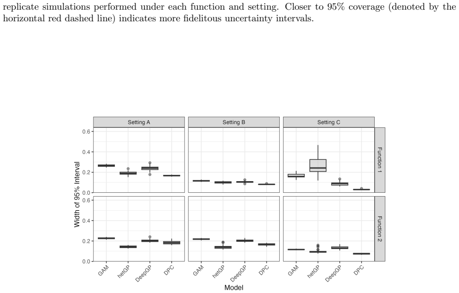
- On simulated data, DPC achieves lower mean squared error than GAM, heteroskedastic GP, and deep GP in 97.7% of replicate-level comparisons, with 95% interval coverage close to nominal.
- The adaptive bandwidth $\sigma$ differentiates linear and nonlinear regions of the power spectrum: small values in the BAO wiggle region and large values in smoother regions at low and high $k$.
- A public R package, 'dpc', implements the MCMC in C and parallelizes the likelihood computation, so other scientists can apply the method to non-cosmological multi-resolution data.
- The model's ability to pool information across related functions means it is most advantageous when many related functions are available; its advantage shrinks when fewer functions are observed.
Reading between the lines
- If the shared second-layer bandwidth is the main source of improvement, the method should transfer to other multi-resolution settings, such as combining low- and high-resolution climate or medical imaging data; a natural ablation test would compare a model with a shared $v$ against one with function-specific bandwidth processes.
- The known-variance assumption is the fragile point: with variances estimated from the data and treated as fixed, credible intervals may be miscalibrated; a natural extension is to place priors on the precision parameters and propagate their uncertainty.
- The observed LR/HR residual trend suggests the model could absorb a constant vertical offset $\Delta$ at the join points rather than smooth through it; inferring $\Delta$ in the posterior would quantify the box-size bias instead of leaving it in the residuals.
- Coverage claims are conditional on the simulation design; a broader test across many more synthetic function families, including functions with genuinely different degrees of wiggliness, would clarify how universal the 95.1% average coverage is.
Editorial analysis
A structured set of objections, weighed in public.
Referee Report
Summary. The paper introduces a Bayesian deep process convolution (DPC) model for estimating nonstationary functions from noisy multi-resolution realizations. The model places a process convolution prior on a latent Brownian motion process, with a second convolution layer controlling the bandwidth as a function of the input, thereby allowing smoothness to vary across the domain and to be shared across related functions. The first-layer latent processes are integrated out, producing an MCMC sampler over the bandwidth latent vector and variance parameters (Lemma 2.1). The method is benchmarked on synthetic data generated from two analytic functions under three noise settings and compared against GAMs, heteroskedastic Gaussian processes, and deep Gaussian processes; it is then applied to the Mira-Titan matter power spectrum data. An R package implementing the method is released.
Significance. If the simulation results are valid, the DPC model is a useful addition to the toolbox for nonstationary, multi-resolution emulation, and the release of an R package plus the explicit marginalization lemma are concrete contributions. The simulation protocol correctly avoids circularity by generating data from analytic functions rather than from the DPC model, and the cosmological application demonstrates a plausible real use case. However, the central empirical claim of superior accuracy and uncertainty quantification rests on a comparison in which DPC appears to be given the true generative noise precisions while competitors must estimate them; the cosmological application does not have such oracle information. This is a load-bearing issue that must be addressed before the headline claim can be accepted.
major comments (2)
- [§3.1 and §4.1, Eq. (4)] The simulation comparison is asymmetric: the DPC model is given the true per-point noise precisions while the competitors (GAM, hetGP, DeepGP) must estimate the noise from the data. Section 2.2 fixes Ω_ij as known, and Section 3.1 specifies the generative standard deviations σ1(x) and σ2(x); the paper never states that DPC used estimated variances in the simulation, and the natural implementation uses the true precisions. This information advantage could explain the DPC's lower MSE and the unusually clean 95.1% average coverage in Figures 6–8, without implying that the DPC construction itself is superior. Please state explicitly what variances DPC was given in the simulations; if it was given the true generating variances, rerun the comparison with matched information (for example, estimate variances for DPC as well, or supply the true variances to all methods) and report whether the MSE and coverage advantages persist.
- [§3.2] The cosmological application does not satisfy the model's assumption of known per-point precisions. In Section 3.2, variances are estimated from theoretical calculations under a log-normality approximation, pooled across cosmologies, and then treated as fixed. If these estimates are biased, for example due to unmodeled low-resolution/high-resolution box-size effects, the credible intervals and coverage reported in Section 4.2 would be misstated. The simulation study therefore validates the model under exactly the condition that the real application cannot meet, and it does not establish that the reported cosmological credible intervals are calibrated. Please add a sensitivity analysis that perturbs the estimated variances or propagates their uncertainty, or explicitly restrict the claims to the known-variance setting.
minor comments (7)
- [§2.1, Eq. (2)] The notation ∫_{S_x} k(x_i - s) y(x_i) dx is not well-defined for a discrete set S_x; the expression should be written as a summation or as a convolution with respect to a discrete measure.
- [§2.2, Lemma 2.1] The exponent nnu/2 in the marginal posterior is undefined; it presumably means n n_u / 2, the total number of latent u entries, and should be defined explicitly.
- [§2.2] The statement that all elements of σ = K_δ v must be positive is not accompanied by a mechanism such as a truncated prior or a transformation; the posterior expression and the MCMC description do not indicate how this restriction is enforced. If the restriction is not enforced, the model is sign-symmetric and the issue should be discussed; if it is enforced, the implementation should be described.
- [§3.2] The notation P(k) = log_{10}(k^{1.5} P(k) / 2π^2) uses P for both the original and the transformed spectrum; please introduce a distinct symbol for the transformed quantity to avoid confusion.
- [§4.1] The text contains a typo, 'summarizing the the coverage'; also, 'an exception being' should be 'an exception being' with correct article usage.
- [§3.1] The main text does not state the number of observations per function and replicate, the number of latent grid points for u and v, or the MCMC settings used in the simulation; these details should be provided or more specifically referenced in the Supplemental Materials.
- [§4.2] The MCMC diagnostics are described only as 'satisfactory'; please report effective sample sizes or convergence statistics, or clearly state that they are in the Supplemental Materials.
Circularity Check
No significant circularity: the DPC posterior is derived from a stated likelihood and priors, and the simulation benchmarks use externally generated functions, so the central claims do not reduce to the model's own inputs.
full rationale
The paper's derivation chain is a standard Bayesian hierarchical model: the likelihood for each realization assumes a known precision matrix Omega_ij, the mean functions are modeled as process convolutions P_i = K_sigma u_i, the bandwidth is itself a convolution sigma = K_delta v, and priors are placed on the hyperparameters. Lemma 2.1 marginalizes the latent u_i analytically; none of these steps defines the target quantity in terms of the answer. The simulation study in Section 3.1 generates data from analytic functions f1 and f2 with added noise, not from the DPC model, so the MSE and coverage comparisons are external to the model's assumptions. The cosmological application in Section 3.2 estimates noise variances from theoretical calculations, pools them across cosmologies, and treats them as fixed; this is a plug-in approximation that could affect interval calibration, but it does not make the estimated mean spectrum identical to the variance input. The paper also candidly discusses unresolved grid-density artifacts in the Discussion, which supports rather than undermines its independence. The main caveat is that Section 2.2 assumes Omega_ij is known; if the Section 4.1 simulations supplied the true generative noise variances to DPC while competitors had to estimate noise, the comparison would be an information asymmetry, but that is a potential experimental-design confound, not a circular derivation, and the paper never states that the true variances were used. No load-bearing self-citation chain is present: prior Coyote/Mira-Titan papers are cited for context, while the present evaluation is self-contained.
Assumptions & free parameters
free parameters (4)
- Prior hyperparameters alpha_u, beta_u, alpha_v, beta_v =
alpha_u = alpha_v = 1, beta_u = beta_v = 0.001
- Upper bound for second-layer bandwidth delta =
delta_max = 10 (default)
- Grid density and locations for latent processes u and v =
Evenly spaced grids; counts m and nv not fixed in paper
- Variance and precision estimates for cosmological data =
Pooled theoretical variances transformed via the sigma-hat-squared formula
assumptions (5)
- domain assumption The power spectrum at the emulation scale is a smooth, nonstationary function with a distinct BAO region of higher wiggliness.
- domain assumption The PT, LR, and HR simulation outputs are unbiased within their specified k cutoffs (k < 0.04 for PT, k < 0.25 for LR, k < 5 for HR).
- domain assumption The log-normal approximation for transforming theoretical variances to the log scale is accurate enough to treat the resulting precision matrix as known.
- domain assumption A Brownian motion latent process provides more stable tail behavior than i.i.d. Gaussian variates for the process convolution.
- standard math Standard linear-Gaussian marginalization (Lemma 2.1) is correctly applied to integrate out the latent u_i.
Cite this review
Pith. "Pith review of Bayesian "Deep" Process Convolutions: An Application in Cosmology." pith.science (2026). https://pith.science/paper/3GELDFLZ
@misc{pith2026241114747,
  author       = {Pith},
  title        = {Pith review of: Bayesian "Deep" Process Convolutions: An Application in Cosmology},
  year         = {2026},
  howpublished = {\url{https://pith.science/paper/3GELDFLZ}},
  note         = {Machine review of arXiv:2411.14747}
}
read the original abstract
The nonlinear matter power spectrum in cosmology describes how matter density fluctuations vary with scale in the universe, providing critical insights into large-scale structure formation. The matter power spectrum includes both smooth regions and highly oscillatory features. Cosmologists rely on noisy, multi-resolution realizations of large N-body simulations to study these phenomena, which require appropriate smoothing techniques to learn about underlying structures. We introduce a Bayesian Deep Process Convolution (DPC) model that flexibly adapts its smoothness parameter across the input space, enabling it to capture both smooth and variable structure within a single framework. The DPC model leverages common patterns across related functions to improve estimation in regions with sparse data. Compared to existing methods, the DPC model offers superior accuracy and uncertainty quantification in simulated data, and qualitatively superior performance with the cosmological data. This methodology will be useful in cosmology and other fields requiring flexible modeling of smooth nonstationary surfaces.
Figures


Figures from the paper (10 more)




Reference graph
Works this paper leans on
-
[1]
Gramacy, R. B. and Lee, H. K. H. (2008). B ayesian treed G aussian process models with an application to computer modeling. Journal of the American Statistical Association , 103(483):1119--1130
work page 2008
-
[2]
Heitmann, K., Bingham, D., Lawrence, E., Bergner, S., Habib, S., Higdon, D., Pope, A., Biswas, R., Finkel, H., Frontiere, N., et al. (2016). The Mira -- Titan universe: P recision predictions for dark energy surveys. The Astrophysical Journal , 820(2):108
work page 2016
-
[3]
J., Lawrence, E., and Wagner, C
Heitmann, K., Higdon, D., White, M., Habib, S., Williams, B. J., Lawrence, E., and Wagner, C. (2009). The coyote universe. II . C osmological models and precision emulation of the nonlinear matter power spectrum. The Astrophysical Journal , 705(1):156
work page 2009
-
[4]
Heitmann, K., White, M., Wagner, C., Habib, S., and Higdon, D. (2010). The coyote universe. I . P recision determination of the nonlinear matter power spectrum. The Astrophysical Journal , 715(1):104
work page 2010
-
[5]
Higdon, D., Swall, J., and Kern, J. (2022). Non-stationary spatial modeling. arXiv preprint arXiv:2212.08043
work page Pith review arXiv 2022
-
[6]
Lawrence, E., Heitmann, K., Kwan, J., Upadhye, A., Bingham, D., Habib, S., Higdon, D., Pope, A., Finkel, H., and Frontiere, N. (2017). The Mira -- Titan universe. II . M atter power spectrum emulation. The Astrophysical Journal , 847(1):50
work page 2017
-
[7]
Lawrence, E., Heitmann, K., White, M., Higdon, D., Wagner, C., Habib, S., and Williams, B. (2010). The coyote universe. III . S imulation suite and precision emulator for the nonlinear matter power spectrum. The Astrophysical Journal , 713(2):1322
work page 2010
-
[8]
Moran, K. R., Heitmann, K., Lawrence, E., Habib, S., Bingham, D., Upadhye, A., Kwan, J., Higdon, D., and Payne, R. (2023). The Mira -- Titan universe-- IV . H igh-precision power spectrum emulation. Monthly Notices of the Royal Astronomical Society , 520(3):3443--3458
work page 2023
Show all 11 references
-
[9]
and Deisenroth, M
Salimbeni, H. and Deisenroth, M. (2017). Doubly stochastic variational inference for deep Gaussian processes. Advances in neural information processing systems , 30
2017
-
[10]
M., and Nobre, A
Sans \'o , B., Schmidt, A. M., and Nobre, A. A. (2008). Bayesian spatio-temporal models based on discrete convolutions. Canadian Journal of Statistics , 36(2):239--258
2008
-
[11]
Sauer, A., Cooper, A., and Gramacy, R. B. (2023). Vecchia-approximated deep Gaussian processes for computer experiments. Journal of Computational and Graphical Statistics , 32(3):824--837
2023
Reviewed August 12, 2026 · model on record in the stance chip above.
Discussion (0). Continue with ORCID to comment.