REVIEW 2 major objections 6 minor 62 references
Downlink MIMO Channel Estimation from Bits: Recoverability and Algorithm
T0 review · 2 major / 6 minor · reviewed 2026-08-12 · deepseek-v4-flash
Pith's one-line read The paper proves that dithered, quantized random projections of a K-path MIMO channel are enough for the base station to recover the full channel, with mean-squared error that decays as the reciprocal of the square root of the number of…
desk verdict Solid Scheme 1 theory and a strong algorithm, but Theorem 2's normalization error sinks the Scheme 2 recoverability claim as stated. read the letter →
The pith
A machine-rendered reading of the paper's core claim, the machinery that carries it, and where it could break.
The reading
What carries the argument
The central objects are the channel manifold $\Gamma$ (all channel matrices generated by $K$ AoAs, $K$ AoDs, and $K$ complex path losses under ULA steering vectors) and the random linear maps that compress it: the Gaussian matrix $A$ in Scheme 1 and the Khatri-Rao product matrix $D$ in Scheme 2. The proof pipeline has four load-bearing pieces: covering-number control of $\Gamma$, which bounds the complexity of the candidate set; a set-restricted eigenvalue (S-REC) condition on the measurement matrix, which turns closeness in the compressed domain into closeness in the channel domain; a KL-divergence/Hellinger link for the dithered quantizer, which converts excess likelihood loss into Euclidean error; and, for Scheme 2 only, a JL-moment property for $D$ plus a spectral-norm bound. On the algorithmic side, the MLE is solved by an ADMM method whose $z$-subproblem is a two-dimensional harmonic retrieval problem, attacked by a modified RELAX routine (discrete Fourier initialization followed by gradient refinement), and whose $H$-subproblem is a closed-form EM update.
What would settle it
Numerically estimate the covering number $C(\Gamma,\epsilon)$ by gridding the parameter space $(\theta,\phi,\beta)$ for $K = 3,\ldots,8$ and computing the smallest radius-$\epsilon$ net of the channel manifold; if $\log C(\Gamma,\epsilon)$ grows like $4K\log(1/\epsilon)$ rather than $2K\log(1/\epsilon)$, the union bound behind Theorem 1 would require more than $\Omega(K\log K)$ measurements. Running Scheme 2 with exactly the implemented distributions $a_t \sim \mathcal{N}(0,I/T^2)$ and $s_t \sim \mathcal{CN}(0,I)$ and checking whether the MSE follows the $O(1/\sqrt{T})$ curve at the $K^2\log^2 K$ threshold would settle whether the proven guarantee covers the implemented algorithm.
Extended reading notes
Core claim
Under the double directional model $H = \sum_{k=1}^K \beta_k a_r(\theta_k) a_t(\phi_k)^H$ with $K$ propagation paths, the paper establishes that the channel is identifiable from dithered uniform-quantized random projections. In Scheme 1 the user forms a least-squares channel estimate, compresses it with a Gaussian matrix $A$ whose entries are $\mathcal{N}(0,1/R)$, and feeds back the quantized bits; Theorem 1 proves that when $R = \Omega(K\log(\sqrt{\kappa}\,L_G K))$, the MLE $h^\star$ satisfies $\|h^{\natural} - h^\star\|_2^2/(MN) \le (64/\sqrt{R})(4L_f/F_f(\tau + 3\nu/4) + 9U_f/F_f\sqrt{2\log(2/\eta)}) + 32\psi^2/R$ with probability at least $1 - 3\eta - \vartheta - e^{-\Omega(R)}$. Theorem 2 gives the same type of bound for the scheme that compresses the raw received pilots, at the higher cost $T = \Omega(K^2\log^2(\sqrt{\kappa}\,L_G K))$. The dithering level enters through the ratios $L_f/F_f$ and $U_f/F_f$, so the theorems quantify why too little dithering leaves quantization noise correlated while too much dithering overwhelms the signal.
Load-bearing premise
The whole result rests on the channel set being small enough in a precise geometric sense and on the random measurement matrices never collapsing the distance between two different channels; if either assumption fails, the advertised $K\log K$ and $K^2\log^2 K$ feedback budgets are not guaranteed.
Editorial extensions
If this is right
- Feedback overhead scales with the number of propagation paths $K$ rather than with the antenna counts $M$ and $N$, so enlarging the array does not inflate the bit budget under the double directional model.
- At a fixed measurement budget $G$, both schemes have the same normalized-MSE upper bound, but Scheme 1 supports $K = O(G)$ paths while Scheme 2 supports only $K = O(\sqrt{G})$; the user-side computational savings of Scheme 2 come at the price of a narrower recoverability region.
- The normalized MSE decays as $O(1/\sqrt{R})$ in Scheme 1 and $O(1/\sqrt{T})$ in Scheme 2, giving a predictable rule for sizing feedback budgets for a target accuracy.
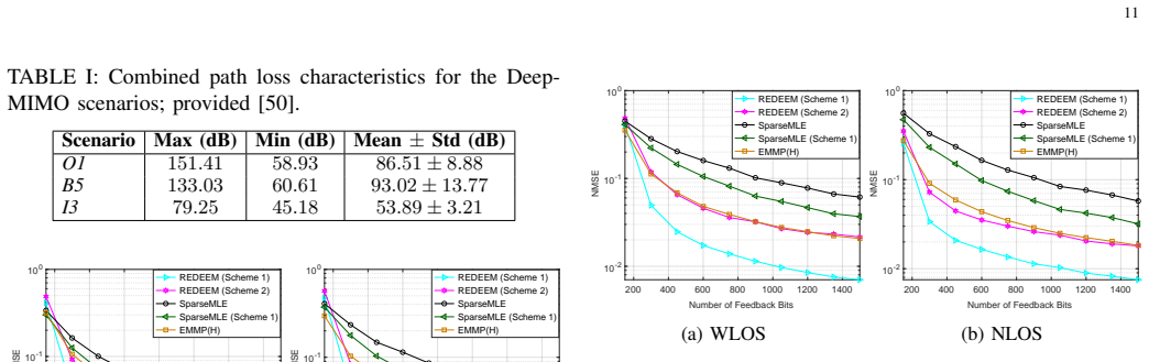
- The REDEEM algorithm, ADMM with a modified RELAX harmonic-retrieval step and an EM quantized-likelihood step, reaches normalized mean-squared errors near $2\times10^{-2}$ at 500 feedback bits in the basic setting, below the dictionary-based baselines, and keeps its advantage in ray-tracing scenarios.
Reading between the lines
- A natural extension the paper leaves open is replacing the random compression matrices with signal-adaptive or learned ones; the same MLE-plus-ADMM construction would carry over, but the S-REC or JL-moment property would need to be re-certified for the new measurement distribution.
- Because the estimator is likelihood-based, one-bit or non-uniform quantizers should fit the same construction: as long as the dithering distribution is known, the KL-to-Hellinger step should yield analogous rates with a modified constant $F_f$.
- The robustness experiment with mis-specified $K$ suggests that over-estimating $K$ is nearly harmless while under-estimating it fails; an implementation could start with a generous path count and prune paths with negligible estimated gains.
- The harmonic-retrieval view of the $z$-subproblem should transfer to other array geometries and to mmWave channels, since only the steering-vector structure and the K-path sum enter the algorithm.
Editorial analysis
A structured set of objections, weighed in public.
Referee Report
Summary. The paper studies limited-feedback downlink channel estimation in FDD massive MIMO. The UE compresses channel information using a random linear map and applies Gaussian-dithered uniform quantization; the BS solves a maximum-likelihood problem over the double-directional channel manifold. Two compression schemes are analyzed: Scheme 1 compresses an LS channel estimate, and Scheme 2 compresses the received pilot signal directly. Recoverability theorems are stated for both schemes, with sample complexity growing as O(K log K) and O(K^2 log^2 K) respectively, where K is the number of propagation paths. The paper also proposes an ADMM algorithm, REDEEM, that combines a modified RELAX harmonic-retrieval solver with an EM step, and reports extensive numerical results on synthetic and DeepMIMO channels.
Significance. The problem is important and the proposed pipeline is a meaningful step beyond dictionary-based sparse recovery: the recoverability analysis via KL/Hellinger divergence together with a set-restricted eigenvalue condition for a parametric channel manifold is a nontrivial extension of quantized compressive sensing. The REDEEM algorithm is a practical contribution, and the experiments show consistent gains over several baselines. However, the Scheme 2 recoverability guarantee is invalid as stated because of a normalization error in the measurement matrix, and the Scheme 1 bound, while correct as an inequality, is too weak to support the advertised sample-complexity claim without an additional J-dependent condition. The core ideas are sound and likely repairable, but the theoretical claims need substantial reworking.
major comments (2)
- [Section IV.C; Appendices F-H (Theorem 2, Lemmas 2-5)] The matrix D defined in Lemma 2 as D=(1/T)(S^T \odot A^T)^T with S\in R^{2N\times T}, A\in R^{2M\times T} has two problems. First, the dimensions do not match: (S^T\odot A^T)^T is (4MN)\times T, while D is claimed to be T\times(4MN); the intended object is presumably (S\odot A)^T with rows (1/T)(s_t^T\otimes a_t^T). Second, with the intended rows and standard-normal s_t,a_t, for any fixed real vector x one has E[(s_t^T X a_t)^2]=\|X\|_F^2=\|x\|_2^2, so E\|Dx\|_2^2=\|x\|_2^2/T, not \|x\|_2^2. Therefore Lemma 3's JL-moment property with mean 1 is false, and Lemma 2's S-REC with \gamma>0 independent of T cannot hold because the expected gain of D on any nonzero vector decays as 1/\sqrt{T}. The implemented Scheme 2 in Section III.B uses a_t\sim N(0,I/T^2), making the actual operator even smaller. The recoverability guarantee for Scheme 2 is thus unsupported as stated; the proof must be redone with a near-isometric normalization, e.g., D=(S\odot A)^T/\sqrt{T} (equivalently a_t\sim N(0,I/T) in the implementation). Note also that Lemma 5's D distribution (entries N(0,1/T)) is inconsistent with Lemma 2's definition.
- [Section IV.B-C; Appendix C (Theorems 1-2, Remark 3)] Even for Scheme 1, where the measurement normalization is correct, the stated bound does not deliver the advertised O(1/\sqrt{R}) rate under the condition R=\Omega(K\log K). The theorem's bound contains \tau=4(2+\sqrt{J/R})+12\sqrt{4K\log(...)}, whose first term contributes O(\sqrt{J/R}/\sqrt{R})=O(\sqrt{J}/R) to the final MSE. Unless R=\Omega(\sqrt{J}) (or a sharper Rademacher bound is used), the error is not O(1/\sqrt{R}), and the claim that performance is insensitive to M and N is not supported by the theorem as stated. In Appendix C, the proof fixes \mu=2+\sqrt{J/R} in the bound \xi(S)\le(4\mu+12\sqrt{\log C(S,\mu)})/\sqrt{R}; choosing \mu\approx\sqrt{K} instead gives a bound of order \sqrt{K\log(J/R)}/\sqrt{R}, which is much milder and restores the intended scaling up to logarithmic factors. The theorem statements and Remark 3 should be revised to either state the additional condition R=\Omega(\sqrt{J}) (respectively T=\Omega(\sqrt{J})) or incorporate the sharper Rademacher argument.
minor comments (6)
- [Fact 2 and Appendix B] The covering-number exponent in Fact 2 is not dimensionally wrong: (8\pi\kappa/\epsilon^2)^{2K} equals (8\pi\kappa)^{2K}\epsilon^{-4K}, so the \epsilon-scaling correctly reflects the 4K real parameters (\theta,\phi,\Re\beta,\Im\beta). The notation is easy to misread, so the authors may wish to write the \epsilon-exponent explicitly.
- [Theorem 1; Appendix C] The proof uses the fact R\le 4MN, which follows from R\le J=2MN by the construction R\ll J, but the theorem statement does not mention this elementary condition; adding one sentence would improve clarity.
- [Theorem 1 and Theorem 2] The statements refer to 'x_i for all i' without defining x_i in the theorem; these should be (Ah)_i and (D\check h)_i in Schemes 1 and 2 respectively.
- [Section V.B, Eq. (35)] The symbol \phi is used both for the standard normal density in the EM surrogate and for the AoD vector; this is confusing and should be disambiguated (e.g., use \varphi for the density).
- [Appendix I] In the proof of Lemma 4, the displayed probability 'Pr(Dh_2 \le (1+\alpha_i)\|h\|_2)' should read 'Pr(\|Dh\|_2 \le (1+\alpha_i)\|h\|_2)'; also, the decomposition (57) should indicate explicitly that \check h_f is the chain tail.
- [Figure 10(b) and Section VI.A.5] The caption claims an O(1/\sqrt{R}) (or O(1/\sqrt{T})) decay rate; this is only justified in the regime where J/R (respectively J/T) is small, given the \tau dependence discussed above, so a qualifier should be added.
Circularity Check
No significant circularity: the recoverability proofs are self-contained; the Scheme 2 normalization issue is a correctness defect, not a reduction of a claim to its own input.
full rationale
The derivation chain is not circular. Theorem 1 is proven from an explicit dithered-quantization likelihood model, standard concentration tools (Hoeffding, Rademacher complexity, Dudley integral), and an S-REC condition whose only manifold input is the independently derived covering bound of Fact 2 (Appendix B). The constants U_f, L_f, F_f are properties of the quantizer and dither level (equations (21)-(23)), not fitted to the recovered channel; Assumption 1 is an explicit modeling-error slack, not a restatement of the theorem. Theorem 2 uses the same pipeline for the Khatri-Rao measurement matrix D, with the S-REC argument given in Appendices F-J. Author self-citations ([25], [33], [49], [61]) are contextual or accompanied by self-contained proofs relying on external results (e.g., Vershynin's corollary); they are not load-bearing uniqueness theorems. The serious issue in the Scheme 2 theory is a correctness gap, not circularity: with D = (1/T)(S^T ⊙ A^T)^T as stated in Theorem 2/Lemma 2, each row has variance ||x||^2/T^2, so E||Dx||_2^2 = ||x||_2^2/T, whereas Lemma 3's JL-moment property requires E||Dx||_2^2 = ||x||_2^2; the implemented Scheme 2 uses a_t ∼ N(0, I/T^2), which is a different distribution. This unsupported normalization means the advertised Scheme 2 recoverability guarantee is not established as stated, but the flaw is an internal inconsistency/unsupported lemma rather than a circular derivation.
Assumptions & free parameters
free parameters (4)
- Model order K =
6 in most experiments
- Dithering level sigma_v =
25% of maximal signal amplitude
- Quantization boundaries =
min and max of 1000 historic CSI samples
- ADMM penalty rho =
1
assumptions (6)
- domain assumption The true channel satisfies H = sum_{k=1}^K beta_k a_r(theta_k) a_t(phi_k)^H with known K and |beta_k| <= kappa.
- domain assumption Assumption 1: min_{z in Z} ||G(z) - H_true||_F <= nu for some nu >= 0.
- domain assumption G is L_G-Lipschitz with finite constant L_G.
- standard math A random Gaussian matrix with entries N(0,1/R) satisfies JL norm preservation, the spectral norm bound (48), and S-REC over Gamma.
- standard math The Khatri-Rao product matrix D = (1/T)(S^T circle A^T)^T satisfies the JL-moment property and the spectral norm bound in Lemma 5.
- domain assumption For bounded x_i, the quantized likelihood has bounded log-likelihood U_f, bounded derivative ratio L_f, and positive curvature F_f uniformly over quantization cells.
Cite this review
Pith. "Pith review of Downlink MIMO Channel Estimation from Bits: Recoverability and Algorithm." pith.science (2026). https://pith.science/paper/2W3OTRBA
@misc{pith2026241116043,
  author       = {Pith},
  title        = {Pith review of: Downlink MIMO Channel Estimation from Bits: Recoverability and Algorithm},
  year         = {2026},
  howpublished = {\url{https://pith.science/paper/2W3OTRBA}},
  note         = {Machine review of arXiv:2411.16043}
}
read the original abstract
In frequency division duplex (FDD) massive MIMO systems, a major challenge lies in acquiring the downlink channel state information}\ (CSI) at the base station (BS) from limited feedback sent by the user equipment (UE). To tackle this fundamental task, our contribution is twofold: First, a simple feedback framework is proposed, where a compression and Gaussian dithering-based quantization strategy is adopted at the UE side, and then a maximum likelihood estimator (MLE) is formulated at the BS side. Recoverability of the MIMO channel under the widely used double directional model is established. Specifically, analyses are presented for two compression schemes -- showing one being more overhead-economical and the other computationally lighter at the UE side. Second, to realize the MLE, an alternating direction method of multipliers (ADMM) algorithm is proposed. The algorithm is carefully designed to integrate a sophisticated harmonic retrieval (HR) solver as subroutine, which turns out to be the key of effectively tackling this hard MLE problem.Extensive numerical experiments are conducted to validate the efficacy of our approach.
Figures


Figures from the paper (7 more)



Reference graph
Works this paper leans on
-
[1]
Goldsmith,Wireless Communications
A. Goldsmith,Wireless Communications. Cambridge University Press, 2005
2005
-
[2]
An overview of limited feedback in wireless commu- nication systems,
D. J. Love, R. W. Heath, V . K. N. Lau, D. Gesbert, B. D. Rao, and M. Andrews, “An overview of limited feedback in wireless commu- nication systems,”IEEE J. Sel. Areas Commun., vol. 26, no. 8, pp. 1341–1365, 2008
work page 2008
-
[3]
MIMO broadcast channels with finite-rate feedback,
N. Jindal, “MIMO broadcast channels with finite-rate feedback,”IEEE Trans. Inf. Theory, vol. 52, no. 11, pp. 5045–5060, 2006
2006
-
[4]
Energy and spectral effi- ciency of very large multiuser MIMO systems,
H. Q. Ngo, E. G. Larsson, and T. L. Marzetta, “Energy and spectral effi- ciency of very large multiuser MIMO systems,”IEEE Trans. Commun., vol. 61, no. 4, pp. 1436–1449, 2013
2013
-
[5]
Spatially common sparsity based adaptive channel estimation and feedback for FDD massive MIMO,
Z. Gao, L. Dai, Z. Wang, and S. Chen, “Spatially common sparsity based adaptive channel estimation and feedback for FDD massive MIMO,” IEEE Trans. Signal Process., vol. 63, no. 23, pp. 6169–6183, 2015
work page 2015
-
[6]
An overview of massive MIMO: Benefits and challenges,
L. Lu, G. Y . Li, A. L. Swindlehurst, A. Ashikhmin, and R. Zhang, “An overview of massive MIMO: Benefits and challenges,”IEEE J. Sel. Topics Signal Process., vol. 8, no. 5, pp. 742–758, 2014
2014
-
[7]
Achievable rates of FDD massive MIMO systems with spatial channel correlation,
Z. Jiang, A. F. Molisch, G. Caire, and Z. Niu, “Achievable rates of FDD massive MIMO systems with spatial channel correlation,”IEEE Trans. Wireless Commun., vol. 14, no. 5, pp. 2868–2882, 2015
work page 2015
-
[8]
Channel estimation for FDD massive MIMO OFDM systems,
D. Hu and L. He, “Channel estimation for FDD massive MIMO OFDM systems,” inProc. IEEE 86th Veh. Tech. Conf. (VTC-Fall). IEEE, 2017, pp. 1–5
work page 2017
Show all 62 references
-
[9]
Pushing the limit of Type I codebook for FDD massive MIMO beamforming: A channel covariance reconstruction approach,
K. Li, Y . Li, L. Cheng, Q. Shi, and Z.-Q. Luo, “Pushing the limit of Type I codebook for FDD massive MIMO beamforming: A channel covariance reconstruction approach,” inProc. IEEE Int. Conf. Acoustics, Speech, Signal Process. (ICASSP), 2021, pp. 4785–4789
2021
-
[10]
CSI sensing from heterogeneous user feedbacks: A constrained phase retrieval approach,
L. Li, X. Zeng, Y .-F. Liu, Y . Xu, and T.-H. Chang, “CSI sensing from heterogeneous user feedbacks: A constrained phase retrieval approach,” IEEE Trans. Wireless Commun., vol. 22, no. 10, pp. 6930–6945, 2023
2023
-
[11]
On the performance of random vector quantization limited feedback beamforming in a MISO system,
C. K. Au-yeung and D. J. Love, “On the performance of random vector quantization limited feedback beamforming in a MISO system,”IEEE Trans. Wireless Commun., vol. 6, no. 2, pp. 458–462, 2007
2007
-
[12]
Noncoherent trellis coded quantization: A practical limited feedback technique for massive MIMO systems,
J. Choi, Z. Chance, D. J. Love, and U. Madhow, “Noncoherent trellis coded quantization: A practical limited feedback technique for massive MIMO systems,”IEEE Trans. Commun., vol. 61, no. 12, pp. 5016–5029, 2013
2013
-
[13]
Distributed compressive CSIT estimation and feedback for FDD multi-user massive MIMO systems,
X. Rao and V . K. N. Lau, “Distributed compressive CSIT estimation and feedback for FDD multi-user massive MIMO systems,”IEEE Trans. Signal Process., vol. 62, no. 12, pp. 3261–3271, 2014
2014
-
[14]
Limited feedback channel estimation in massive MIMO with non- uniform directional dictionaries,
P. N. Alevizos, X. Fu, N. D. Sidiropoulos, Y . Yang, and A. Bletsas, “Limited feedback channel estimation in massive MIMO with non- uniform directional dictionaries,”IEEE Trans. Signal Process., vol. 66, no. 19, pp. 5127–5141, 2018
2018
-
[15]
Sparse channel estimation for massive MIMO with 1-bit feedback per dimension,
Z. Zhou, X. Chen, D. Guo, and M. L. Honig, “Sparse channel estimation for massive MIMO with 1-bit feedback per dimension,” inProc. 2017 IEEE Wireless Communi. Netw. Conf. (WCNC). IEEE, 2017, pp. 1–6
2017
-
[16]
Algebraic channel estimation algorithms for FDD massive MIMO systems,
C. Qian, X. Fu, and N. D. Sidiropoulos, “Algebraic channel estimation algorithms for FDD massive MIMO systems,”IEEE J. Sel. Topics Signal Process., vol. 13, no. 5, pp. 961–973, 2019
2019
-
[17]
Integrated sensing and communication with massive MIMO: A unified tensor approach for channel and target parameter estimation,
R. Zhang, L. Cheng, S. Wang, Y . Lou, Y . Gao, W. Wu, and D. W. K. Ng, “Integrated sensing and communication with massive MIMO: A unified tensor approach for channel and target parameter estimation,” IEEE Trans. Wireless Commun., vol. 23, no. 8, pp. 8571–8587, 2024
2024
-
[18]
Compressive sensing based channel feedback protocols for spatially-correlated massive antenna arrays,
P.-H. Kuo, H. T. Kung, and P.-A. Ting, “Compressive sensing based channel feedback protocols for spatially-correlated massive antenna arrays,” inProc. IEEE Wireless Communi. Netw. Conf. (WCNC). IEEE, 2012, pp. 492–497
2012
-
[19]
Tensor-based channel estimation for dual-polarized massive MIMO systems,
C. Qian, X. Fu, N. D. Sidiropoulos, and Y . Yang, “Tensor-based channel estimation for dual-polarized massive MIMO systems,”IEEE Trans. Signal Process., vol. 66, no. 24, pp. 6390–6403, 2018
2018
-
[20]
Compressed channel sensing: A new approach to estimating sparse multipath chan- nels,
W. U. Bajwa, J. Haupt, A. M. Sayeed, and R. Nowak, “Compressed channel sensing: A new approach to estimating sparse multipath chan- nels,”Proc. IEEE, vol. 98, no. 6, pp. 1058–1076, 2010
2010
-
[21]
FDD massive MIMO channel estimation with arbitrary 2D-array geometry,
J. Dai, A. Liu, and V . K. Lau, “FDD massive MIMO channel estimation with arbitrary 2D-array geometry,”IEEE Trans. Signal Process., vol. 66, no. 10, pp. 2584–2599, 2018
2018
-
[22]
Tensor-based channel esti- mation for millimeter wave MIMO-OFDM with dual-wideband effects,
Y . Lin, S. Jin, M. Matthaiou, and X. You, “Tensor-based channel esti- mation for millimeter wave MIMO-OFDM with dual-wideband effects,” IEEE Trans. Commun., vol. 68, no. 7, pp. 4218–4232, 2020
2020
-
[23]
Channel estimation and hybrid precoding for millimeter wave cellular systems,
A. Alkhateeb, O. El Ayach, G. Leus, and R. W. Heath, “Channel estimation and hybrid precoding for millimeter wave cellular systems,” IEEE J. Sel. Topics Signal Process., vol. 8, no. 5, pp. 831–846, 2014
2014
-
[24]
Efficient mixed-spectrum estimation with applica- tions to target feature extraction,
J. Li and P. Stoica, “Efficient mixed-spectrum estimation with applica- tions to target feature extraction,”IEEE Trans. Signal Process., vol. 44, no. 2, p. 281–295, 1996
1996
-
[25]
Massive MIMO channel estimation via compressed and quantized feedback,
M. Shao and X. Fu, “Massive MIMO channel estimation via compressed and quantized feedback,” in2022 56th Asilomar Conf. Signals, Syst., Comput., 2022, pp. 1016–1020
2022
-
[26]
An overview of signal processing techniques for millimeter wave MIMO systems,
R. W. Heath, N. Gonz ´alez-Prelcic, S. Rangan, W. Roh, and A. M. Sayeed, “An overview of signal processing techniques for millimeter wave MIMO systems,”IEEE J. Sel. Topics Signal Process., vol. 10, no. 3, pp. 436–453, 2016
2016
-
[27]
Stoica and R
P. Stoica and R. L. Moses,Spectral analysis of signals. Upper Saddle River, N.J.: Pearson/Prentice Hall Upper Saddle River, N.J., 2005
2005
-
[28]
Multidimensional frequency estimation with finite snapshots in the presence of identical frequencies,
J. Liu, X. Liu, and X. Ma, “Multidimensional frequency estimation with finite snapshots in the presence of identical frequencies,”IEEE Trans. Signal Process., vol. 55, no. 11, pp. 5179–5194, 2007
2007
-
[29]
Harmonic retrieval based baseband channel estimation for millimeter wave OFDM systems,
Z. Sha, Z. Wang, and S. Chen, “Harmonic retrieval based baseband channel estimation for millimeter wave OFDM systems,”IEEE Trans. Veh. Tech., vol. 68, no. 3, pp. 2668–2681, 2019
2019
-
[30]
Tensor algebra and multidimensional harmonic retrieval in signal processing for MIMO radar,
D. Nion and N. D. Sidiropoulos, “Tensor algebra and multidimensional harmonic retrieval in signal processing for MIMO radar,”IEEE Trans. Signal Process., vol. 58, no. 11, pp. 5693–5705, 2010
2010
-
[31]
Quantization and dither: A theoretical survey,
S. P. Lipshitz, R. A. Wannamaker, and J. Vanderkooy, “Quantization and dither: A theoretical survey,”J. Audio Engineer. Society, vol. 40, no. 5, pp. 355–375, 1992
1992
-
[32]
A theory of nonsubtractive dither,
R. Wannamaker, S. Lipshitz, J. Vanderkooy, and J. Wright, “A theory of nonsubtractive dither,”IEEE Trans. Signal Process., vol. 48, no. 2, pp. 499–516, 2000
2000
-
[33]
Quantized radio map estimation using tensor and deep generative models,
S. Timilsina, S. Shrestha, and X. Fu, “Quantized radio map estimation using tensor and deep generative models,”IEEE Trans. Signal Process., 2023
2023
-
[34]
R. A. Horn and C. R. Johnson,Topics in Matrix Analysis. Cambridge University Press, 1991
1991
-
[35]
Shalev-Shwartz and S
S. Shalev-Shwartz and S. Ben-David,Understanding Machine Learning: From Theory to Algorithms. USA: Cambridge University Press, 2014
2014
-
[36]
1-bit matrix completion,
M. A. Davenport, Y . Plan, E. van den Berg, and M. Wootters, “1-bit matrix completion,”Inf. Inference: J. IMA, vol. 3, no. 3, pp. 189–223, 2014
2014
-
[37]
Learning tensors from partial binary measurements,
N. Ghadermarzy, Y . Plan, and O. Yilmaz, “Learning tensors from partial binary measurements,”IEEE Trans. Signal Process., vol. 67, no. 1, pp. 29–40, 2018
2018
-
[38]
Tensor denoising and completion based on ordinal observations,
C. Lee and M. Wang, “Tensor denoising and completion based on ordinal observations,” inProc. Int. Conf. Mach. Learn. (ICML). PMLR, 2020, pp. 5778–5788
2020
-
[39]
Spectrum cartography via coupled block-term tensor decomposition,
G. Zhang, X. Fu, J. Wang, X.-L. Zhao, and M. Hong, “Spectrum cartography via coupled block-term tensor decomposition,”IEEE Trans. Signal Process., vol. 68, pp. 3660–3675, 2020
2020
-
[40]
Deep spectrum cartography: Com- pleting radio map tensors using learned neural models,
S. Shrestha, X. Fu, and M. Hong, “Deep spectrum cartography: Com- pleting radio map tensors using learned neural models,”IEEE Trans. Signal Process., vol. 70, pp. 1170–1184, 2022. 15
2022
-
[41]
Robust 1-bit compressed sensing and sparse logistic regression: A convex programming approach,
Y . Plan and R. Vershynin, “Robust 1-bit compressed sensing and sparse logistic regression: A convex programming approach,”IEEE Trans. Inf. Theor., vol. 59, no. 1, p. 482–494, Jan. 2013
2013
-
[42]
Quantization and compressive sensing,
P. T. Boufounos, L. Jacques, F. Krahmer, and R. Saab, “Quantization and compressive sensing,” inProc. Compressed Sensing Its Appl.: MATHEON Workshop. Springer, 2015, pp. 193–237
2015
-
[43]
Quantized compressive sensing with RIP matrices: the benefit of dithering,
C. Xu and L. Jacques, “Quantized compressive sensing with RIP matrices: the benefit of dithering,”Inf. Inference: J. IMA, vol. 9, no. 3, pp. 543–586, 11 2019
2019
-
[44]
Quantization of compressive samples with stable and robust recovery,
R. Saab, R. Wang, and ¨O. Yılmaz, “Quantization of compressive samples with stable and robust recovery,”Applied and Computational Harmonic Analysis, vol. 44, no. 1, pp. 123–143, 2018
2018
-
[45]
Compressed sensing using generative models,
A. Bora, A. Jalal, E. Price, and A. G. Dimakis, “Compressed sensing using generative models,” inProc. Int. Conf. Mach. Learn. (ICML). PMLR, 2017, pp. 537–546
2017
-
[46]
Distributed optimization and statistical learning via the alternating direction method of multipliers,
S. Boyd, N. Parikh, E. Chu, B. Peleato, and J. Eckstein, “Distributed optimization and statistical learning via the alternating direction method of multipliers,”Foundations Trends Mach. Learn., vol. 3, pp. 1–122, 01 2011
2011
-
[47]
Compressed sensing with quan- tized measurements,
A. Zymnis, S. Boyd, and E. Candes, “Compressed sensing with quan- tized measurements,”IEEE Signal Process. Lett., vol. 17, no. 2, pp. 149–152, 2009
2009
-
[48]
Multiple parameter estimation with quantized channel output,
A. Mezghani, F. Antreich, and J. A. Nossek, “Multiple parameter estimation with quantized channel output,” in2010 International ITG Workshop on Smart Antennas (WSA), 2010, p. 143–150
2010
-
[49]
Accelerated and deep expectation maximization for one-bit MIMO-OFDM detection,
M. Shao, W.-K. Ma, J. Liu, and Z. Huang, “Accelerated and deep expectation maximization for one-bit MIMO-OFDM detection,”IEEE Trans. Signal Process., 2024
2024
-
[50]
DeepMIMO: A generic deep learning dataset for mil- limeter wave and massive MIMO applications,
A. Alkhateeb, “DeepMIMO: A generic deep learning dataset for mil- limeter wave and massive MIMO applications,” inProc. of Information Theory and Applications Workshop (ITA), San Diego, CA, Feb 2019, pp. 1–8
2019
-
[51]
Limited feedback double directional massive MIMO channel estimation: From low-rank modeling to deep learning,
H. Sun, Z. Zhao, X. Fu, and M. Hong, “Limited feedback double directional massive MIMO channel estimation: From low-rank modeling to deep learning,” inProc. IEEE 19th Int. Workshop Signal Process. Advances Wireless Commun. (SPAWC), 2018
2018
-
[52]
Channel estimation in millimeter wave MIMO systems with one-bit quantization,
J. Mo, P. Schniter, N. G. Prelcic, and R. W. Heath, “Channel estimation in millimeter wave MIMO systems with one-bit quantization,” inProc. 48th Asilomar Conf. Signals, Syst., Comput.IEEE, 2014, pp. 957–961
2014
-
[53]
Channel estimation in broadband millimeter wave MIMO systems with few-bit ADCs,
J. Mo, P. Schniter, and R. W. Heath, “Channel estimation in broadband millimeter wave MIMO systems with few-bit ADCs,”IEEE Trans. Signal Process., vol. 66, no. 5, pp. 1141–1154, 2018
2018
-
[54]
Wireless InSite,
Remcom, “Wireless InSite,” http://www.remcom.com/wireless-insite
-
[55]
A simple proof of the restricted isometry property for random matrices,
R. Baraniuk, M. Davenport, R. DeV ore, and M. Wakin, “A simple proof of the restricted isometry property for random matrices,”Constructive Approximation, vol. 28, no. 3, p. 253–263, 2008
2008
-
[56]
Spectrally-normalized margin bounds for neural networks,
P. L. Bartlett, D. J. Foster, and M. J. Telgarsky, “Spectrally-normalized margin bounds for neural networks,”Advances Neural Inf. Process. Systems (NeurIPS), vol. 30, 2017
2017
-
[57]
Introduction to the non-asymptotic analysis of random matrices,
R. Vershynin, “Introduction to the non-asymptotic analysis of random matrices,”arXiv preprint arXiv:1011.3027, 2010
2010 arXiv
-
[58]
Categorical matrix completion,
Y . Cao and Y . Xie, “Categorical matrix completion,” inProc. IEEE 6th Int. Workshop Comput. Advances Multi-Sensor Adaptive Process. (CAMSAP). IEEE, 2015, pp. 369–372
2015
-
[59]
R. T. Rockafellar and R. J.-B. Wets,Variational Analysis. Springer Science & Business Media, 2009, vol. 317
2009
-
[60]
Oblivious sketching of high-degree poly- nomial kernels,
T. D. Ahle, M. Kapralov, J. B. Knudsen, R. Pagh, A. Velingker, D. P. Woodruff, and A. Zandieh, “Oblivious sketching of high-degree poly- nomial kernels,” inProc. 14th Annual ACM-SIAM Symposium Discrete Algorithms. SIAM, 2020, pp. 141–160
2020
-
[61]
On recoverability of randomly compressed tensors with low CP rank,
S. Ibrahim, X. Fu, and X. Li, “On recoverability of randomly compressed tensors with low CP rank,”IEEE Signal Process. Lett., vol. 27, pp. 1125– 1129, 2020. 1 Supplementary Material of “Downlink Channel Estima- tion from Compressed and Quantized Feedback” APPENDIXD PER-ITERATI...
2020
-
[62]
In the above, ¯IGA, ¯IEM and ¯IRLX denote the maximum number of iterations for gradient ascent, EM, and Mod-RELAX, respectively
Total per-iteration complexity isO( ¯IEMM N R+ ¯IGA ¯IRLX K 3M N+ ¯IRLX K 2M NlogM N). In the above, ¯IGA, ¯IEM and ¯IRLX denote the maximum number of iterations for gradient ascent, EM, and Mod-RELAX, respectively. Empirically, the algorithm converges in a few iterations. Not...
Reviewed August 12, 2026 · model on record in the stance chip above.
Discussion (0). Continue with ORCID to comment.