REVIEW 3 major objections 4 minor 27 references
Non-Linear Super-Stencils for Turbulence Model Corrections
T0 review · 3 major / 4 minor · reviewed 2026-08-12 · deepseek-v4-flash
Pith's one-line read A neural network that reads a local mean-flow neighborhood can learn a corrective force that brings RANS simulations into close agreement with high-fidelity data, even when trained on a single case and applied to different geometries and…
desk verdict A promising proof-of-concept for nonlocal learned RANS corrections; the transfer results are likely real, but the out-of-sample claim needs a clean validation split and the training target needs independent validation. read the letter →
The pith
A machine-rendered reading of the paper's core claim, the machinery that carries it, and where it could break.
The reading
What carries the argument
The Non-Linear Super-Stencil is the central object: a set of stencil points $x^*_{I,J,K} = c_l s^*_l (I e^*_1/n_1 + J e^*_2/n_2 + K e^*_3/n_3)$ centered at $x^*$, with $s^*_l = \sqrt{k^*}/\omega^*$ the turbulent integral length scale, $e^*_1$ aligned with the local mean velocity, and the whole frame rotated and rescaled to remove orientation and scale variability. At every stencil point the mean velocity, its Lagrangian-shifted value, the strain-rate tensor, the eddy-to-effective viscosity ratio $q = \nu_t/\nu_e$, and a wall indicator are sampled and non-dimensionalized. A residual neural network with an encoder and sixteen residual layers maps the $15\times15\times9$ feature tensor to the dimensionless force $\hat f^*$, which is then re-dimensionalized by $\omega^*\sqrt{k^*}$ and Helmholtz-projected. The stencil's invariance properties are what allow the same network to transfer across geometries and Reynolds numbers.
What would settle it
A direct test would be to construct the exact correction force $f_i$ from Eq. (7), or via a sufficiently large-$\chi$ data-assimilation solve, train the NLSS on that target, and compare its predictions with the relaxation-based network on the same test cases; if the two agree within the reported error reductions, the surrogate bias is negligible, and if they differ, the generalization result would have to be re-evaluated.
Extended reading notes
Core claim
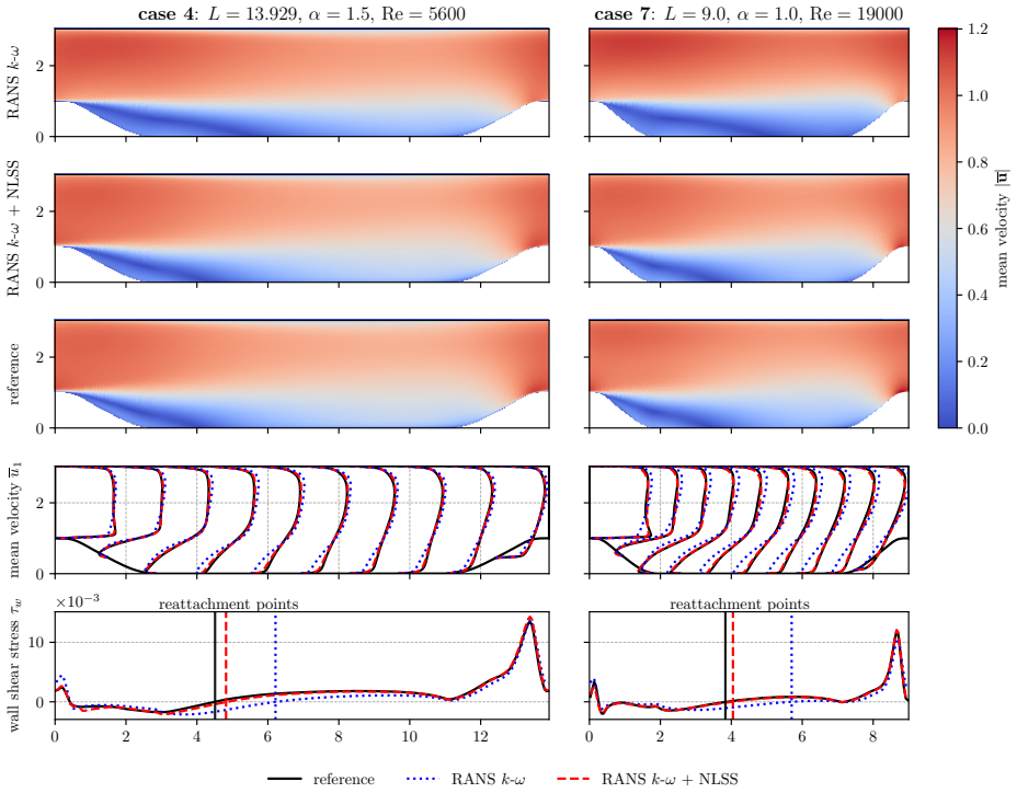
The central discovery claimed is that the correction force $f_i$ in the RANS momentum equation, the difference between the true Reynolds-stress divergence and the eddy-viscosity model, can be expressed as a function of mean-flow data in a compact neighborhood of the point, and that this function is learnable. Training data are produced by solving the RANS equations with a relaxation source term $\chi(\bar u_i^{\text{high fidelity}} - \bar u_i)$ added, with $\chi = \chi_{\max}\min(2q,1)$; at steady state this term approximates the model correction. The inputs are the normalized, rotated, Galilean-transformed stencil samples $\hat u$, $\hat u^{\text{lag}}$, $\hat S$, $q$, and a solid indicator. The paper reports relative $L^2$ mean-velocity errors dropping from e.g. 0.457 to 0.105 (case 4) and 0.515 to 0.128 (case 7) when the trained NLSS correction is applied during RANS solves, with reattachment locations much closer to the reference.
Load-bearing premise
The load-bearing premise is that the relaxation term $\chi(\bar u^{\text{high fidelity}} - \bar u)$ used during training is a faithful stand-in for the true model correction force $f_i$ defined in Eq. (7); the paper's validation compares the network's output to that same relaxation-based extraction, so it does not independently test whether the finite-$\chi$ surrogate is unbiased.
Editorial extensions
If this is right
- Within the periodic-hill family, a single trained NLSS replaces case-by-case RANS calibration, cutting mean-velocity errors by roughly a factor of three to four on unseen geometries and Reynolds numbers.
- Because the correction is force-based and local, the same trained network can in principle be loaded into any k-omega RANS code without retraining on the new grid.
- The method implies that non-local information, not just pointwise strain and rotation features, is what a RANS closure needs to capture separated flows, and that a compact stencil suffices.
- The reported runtime overhead, roughly 20 to 50 times the uncorrected solve, is attributed to stencil-value interpolation, so an optimized sampling implementation would make the approach practical for production RANS.
Reading between the lines
- If the surrogate target is nearly unbiased, the same NLSS pipeline should transfer to other eddy-viscosity models with retraining only, because the force correction absorbs the model's error rather than its specific parameters.
- A testable extension is to train on multiple reference cases simultaneously, which should collapse the remaining error seen in case 1, reattachment on a strongly curved surface, and may reveal whether the network is learning a local pattern library rather than a geometry-specific fit.
- The Galilean- and scale-normalized stencil suggests the learning task is essentially about local dimensionless flow patterns; if so, the same approach could be aimed at other closure problems such as wall heat flux, transition onset, or subgrid stress in coarse LES.
- A strict out-of-family test, such as flow over a backward-facing step or an airfoil, would reveal whether the learned map is a universal local closure or only a hill-family interpolator.
Editorial analysis
A structured set of objections, weighed in public.
Referee Report
Summary. This paper introduces the Non-Linear Super-Stencil (NLSS), a data-driven correction for RANS turbulence models. A fully connected neural network estimates a correction force in the mean momentum equation from non-local, physically normalized flow data sampled on a velocity-aligned, turbulence-length-scale-scaled stencil. Training data are generated for a single periodic-hill LES case by relaxing the RANS solution toward the reference velocity field through a finite-rate source term (Eq. 14). The trained network is then embedded in OpenFOAM's simpleFOAM and applied to seven periodic-hill cases with different geometries and Reynolds numbers. The central claim is that, despite being trained only on case 6, the NLSS-corrected solver produces substantially smaller mean-velocity errors than the uncorrected k-omega model on all test cases (Table 2, e.g., case 4 from 0.457 to 0.105 and case 7 from 0.515 to 0.128).
Significance. If the out-of-sample claim survives scrutiny, the NLSS is a useful proof of concept for non-local, physically normalized data-driven RANS corrections. The method is careful about Galilean invariance and scale alignment, which plausibly reduces the required training data, and the authors provide their implementation in a public repository. At the same time, the paper has two load-bearing ambiguities: the validation/checkpoint-selection protocol and the validation of the relaxation-based training target. The primary support is a posteriori consistency on a small family of flows, so the generalization claim should be read as case-study evidence rather than established methodology.
major comments (3)
- [Section 2.2 and Section 4.2] The training section says 'the model was validated on all cases (1-7) after each epoch', while Section 4.2 says the checkpoint with the lowest validation loss is selected using 'a separate validation set'. If the validation set used for checkpoint selection includes any of the cases later reported as test errors in Table 2, then those test errors are not fully out-of-sample: the epoch is selected on those cases, and the generalization claim is inflated. Please state explicitly whether the validation set was a held-out subset of case 6 or the full set of cases 1-7. If the latter, re-run the experiment with a validation split that excludes all test cases and report Table 2 for the resulting checkpoint.
- [Section 1, Eq. (14), and Section 4.3] The reference force used for training is extracted as f_ref = chi(u_high - u_ref) with chi = chi_max min(2q,1), and the paper does not compare this surrogate with the exact model correction f defined in Eq. (7). The agreement in Fig. 4 is between the trained NLSS and this same relaxation-based extraction, so it does not validate the surrogate itself. If a finite-chi relaxation biases the target, the network learns that bias and the reported generalization rests on an unvalidated training target. I request a convergence/sensitivity test with respect to chi_max (e.g., chi_max = 1, 2, 5, 10 s^{-1}) and, if feasible, an evaluation of the exact f from Eq. (7) on a smooth reference field to check the surrogate's validity.
- [Section 2.1 and Table 4] The paper states that no systematic sensitivity analysis has been performed and that all parameters are heuristic. Given the number of free parameters (chi_max, c_l, c_lag, n_1, n_2, T_NLSS, chi_damp, mu_mem, batch size, learning rate, weight decay), the reported gains could, in principle, depend on a narrow parameter tuning. I ask for at least a one-at-a-time sensitivity study over the most influential parameters (stencil support, Lagrangian shift, relaxation rate, evaluation interval) or an explicit argument why the chosen values are not critical for the principal conclusion.
minor comments (4)
- [Section 1] The sentence 'The standard model parameter values are taken from from [12]' contains a duplicated 'from'.
- [Algorithm 2, line 18] The Helmholtz projection line reads 'phi_f <- solution of nabla^2 phi_f = div f_ref'; in the prediction loop this should be the current predicted force f, not f_ref.
- [Section 4.2, Eq. (19)] The expression 'R^T (u(x - u* delta t, t - delta t)) (delta t omega* sqrt(k*))^{-1}' is missing parentheses for the inverse quantity; the intended meaning is clear but should be written as (delta t omega* sqrt(k*))^{-1} R^T u(...) for clarity.
- [Table 3] The substantial runtime overhead (factors of 20-50) is only briefly attributed to interpolation; a short analysis of the dominant cost would help readers judge the practical relevance of the method.
Circularity Check
Mostly self-contained training and evaluation; the checkpoint-selection ambiguity (validation on all cases 1-7 vs. a separate validation set) partially compromises the out-of-sample claim, but there is no definitional circularity or load-bearing self-citation.
-
fitted input called prediction
[Section 2.2 (Training) and Section 4.2 (Neural network type and architecture)]
"To monitor the model’s accuracy during this process, the model was validated on all cases (1-7) after each epoch. ... During training, the neural network is monitored for over-fitting by evaluating the loss function L on a separate validation set. At the end of the training process, the trained neural network with the lowest validation loss is used for integration into the RANS solver."
Section 2.2 says the model was validated on all cases (1-7) after each epoch, while Section 4.2 selects the checkpoint with the lowest validation loss on a separate validation set. If that validation set includes the same cases 1-7 later reported in Table 2, the checkpoint is chosen by minimizing loss on the test cases, so the reported errors are not fully out-of-sample. The paper never states that the validation set is a held-out subset of the single training case (case 6). This is a selection-on-test effect rather than definitional equivalence, but it fits the pattern of a fitted input (epoch chosen on test cases) being reported as a prediction.
full rationale
The paper's central result is a genuinely supervised, out-of-sample evaluation: the NLSS weights are trained only on case 6 (Section 2.2: 'For training only a single case - namely case 6 - was employed'), and the high-fidelity velocity errors in Table 2 are computed against external DNS/LES data (Xiao et al. [15], Gloerfelt et al. [16]) that do not enter the training objective. The force-extraction surrogate fi ≈ χ(u_hf - u) in Eq. (14) is an acknowledged approximation, not a circular input: the final velocity comparisons are against the true reference fields, and Fig. 4 only demonstrates that the network reproduces the same relaxation-based target it was trained on. Refs [13,14] are prior work from the same group, but they are cited as inspiration for the relaxation ansatz, and the paper gives independent numerical reasons for that choice; no uniqueness claim or load-bearing self-citation is present. The one concrete circularity-adjacent issue is the checkpoint-selection protocol: Section 2.2 says the model was validated on all cases (1-7) after each epoch, while Section 4.2 says the checkpoint with the lowest validation loss on a separate validation set is used. If that validation set is composed of the same cases 1-7 later reported as test cases, then the reported generalization errors are not fully out-of-sample: the epoch is selected using those cases. This is a selection-on-test ambiguity rather than a definitional equivalence, so it does not invalidate the independent content, but it must be resolved (e.g., by stating that the validation set is a held-out subset of case 6) before the generalization claim is clean. Because the core training/test split is otherwise sound, the circularity score is moderate.
Assumptions & free parameters
free parameters (7)
- chi_max (relaxation rate for reference force extraction) =
5 s^-1
- c_l (stencil spatial support factor) =
1.5
- c_lag (Lagrangian shift factor) =
0.1
- n1, n2 (stencil dimensions) =
7, 7
- T_NLSS (correction evaluation interval) =
10 iterations
- chi_damp and mu_mem (solution damping) =
0.5 s^-1, 0.95
- Neural network hyperparameters =
learning rate 3e-4, weight decay 1e-3, batch size 4096, 200 epochs, 5-layer encoder (512-256-128-64-32) + 16 residual…
assumptions (5)
- domain assumption The Boussinesq eddy viscosity hypothesis and the standard k-omega model provide the base turbulence closure that is corrected.
- ad hoc to paper There exists an unambiguous non-linear mapping from the mean flow pattern in a bounded neighborhood of a point to the correction force at that point.
- domain assumption The local turbulent kinetic energy k and frequency omega from the k-omega model are appropriate scales for non-dimensionalization and for defining the stencil size via the integral length scale sqrt(k)/omega.
- standard math The Navier-Stokes equations are Galilean and scale invariant, justifying the velocity alignment, rotation, and normalization of stencil features.
- ad hoc to paper The reference force f_ref obtained from Eq. (14) with finite relaxation chi is a sufficiently accurate substitute for the exact model correction f in Eq. (7).
Cite this review
Pith. "Pith review of Non-Linear Super-Stencils for Turbulence Model Corrections." pith.science (2026). https://pith.science/paper/ZLWKXEBB
@misc{pith2026241116493,
  author       = {Pith},
  title        = {Pith review of: Non-Linear Super-Stencils for Turbulence Model Corrections},
  year         = {2026},
  howpublished = {\url{https://pith.science/paper/ZLWKXEBB}},
  note         = {Machine review of arXiv:2411.16493}
}
read the original abstract
Accurate simulation of turbulent flows remains a challenge due to the high computational cost of direct numerical simulations (DNS) and the limitations of traditional turbulence models. This paper explores a novel approach to augmenting standard models for Reynolds-Averaged Navier-Stokes (RANS) simulations using a Non-Linear Super-Stencil (NLSS). The proposed method introduces a fully connected neural network that learns a mapping from the local mean flow field to a corrective force term, which is added to a standard RANS solver in order to align its solution with high-fidelity data. A procedure is devised to extract training data from reference DNS and large eddy simulations (LES). To reduce the complexity of the non-linear mapping, the dimensionless local flow data is aligned with the local mean velocity, and the local support domain is scaled by the turbulent integral length scale. After being trained on a single periodic hill case, the NLSS-corrected RANS solver is shown to generalize to different periodic hill geometries and different Reynolds numbers, producing significantly more accurate solutions than the uncorrected RANS simulations.
Figures


Figures from the paper (6 more)


Reference graph
Works this paper leans on
-
[1]
O. C. Zienkiewicz, R. L. Taylor, and P. Nithiarasu. Chapter 8 - Turbulent Flows. In O. C. Zienkiewicz, R. L. Taylor, and P. Nithiarasu, editors, The Finite Element Method for Fluid Dynamics (Seventh Edition) , pages 283–308. Butterworth-Heinemann, Oxford, January 2014
work page 2014
-
[2]
P. Spalart. Reflections on RANS Modelling. In Shia-Hui Peng, Piotr Doerffer, and Werner Haase, editors, Progress in Hybrid RANS-LES Modelling , pages 7–24, Berlin, Heidelberg, 2010. Springer
work page 2010
-
[3]
Turbulence Modeling in the Age of Data.Annual Review of Fluid Mechanics , 51(1):357–377, 2019
Karthik Duraisamy, Gianluca Iaccarino, and Heng Xiao. Turbulence Modeling in the Age of Data.Annual Review of Fluid Mechanics , 51(1):357–377, 2019. eprint: https://doi.org/10.1146/annurev-fluid-010518-040547
-
[4]
Yvonne St¨ ocker, Christian Golla, Ramandeep Jain, Jochen Fr¨ ohlich, and Paola Cinnella. DNS-Based Turbulent Closures for Sediment Transport Using Symbolic Regression.Flow, Turbulence and Combustion, 112(1):217–241, January 2024
work page 2024
-
[5]
A wall model for separated flows: embedded learning to improve a posteriori performance
Zhideng Zhou, Xin-lei Zhang, Guo-wei He, and Xiaolei Yang. A wall model for separated flows: embedded learning to improve a posteriori performance, September 2024. arXiv:2409.00984
work page Pith review arXiv 2024
-
[6]
Operator learning of RANS equations: a Graph Neural Network closure model, March 2023
Michele Quattromini, Michele Alessandro Bucci, Stefania Cherubini, and Onofrio Semeraro. Operator learning of RANS equations: a Graph Neural Network closure model, March 2023. arXiv:2303.03806 [physics]
arXiv 2023
-
[7]
Xu-Hui Zhou, Jiequn Han, and Heng Xiao. Frame-independent vector-cloud neural network for nonlocal con- stitutive modeling on arbitrary grids. Computer Methods in Applied Mechanics and Engineering , 388:114211, January 2022
work page 2022
-
[8]
The Graph Neural Network Model
Franco Scarselli, Marco Gori, Ah Chung Tsoi, Markus Hagenbuchner, and Gabriele Monfardini. The Graph Neural Network Model. IEEE Transactions on Neural Networks , 20(1):61–80, January 2009. Conference Name: IEEE Transactions on Neural Networks
work page 2009
Show all 27 references
-
[9]
Reynolds averaged turbulence modelling using deep neural networks with embedded invariance
Julia Ling, Andrew Kurzawski, and Jeremy Templeton. Reynolds averaged turbulence modelling using deep neural networks with embedded invariance. Journal of Fluid Mechanics , 807:155–166, 2016
2016
-
[10]
Boureima, V
I. Boureima, V. Gyrya, J.A. Saenz, S. Kurien, and M. Francois. Dynamic calibration of differential equations using machine learning, with application to turbulence models. Journal of Computational Physics , 457:110924, 2022
2022
-
[11]
Boussinesq
J. Boussinesq. Essai sur la theorie des eaux courantes. In M´ emoires pr´ esent´ es par divers savants ` a l’Acad´ emie des Sciences, XXIII (1) , 1877
-
[12]
David C. Wilcox. Turbulence modeling for cfd. DCW Industries , 2:103–217, 1998. Publisher: La Canada, CA: DCW Industries. 25
1998
-
[13]
Oliver Brenner, Justin Plogmann, Pasha Piroozmand, and Patrick Jenny. A variational data assimilation approach for sparse velocity reference data in coarse rans simulations through a corrective forcing term.Computer Methods in Applied Mechanics and Engineering , 427:117026, 2024
2024
-
[14]
Variational assimilation of sparse time-averaged data for efficient adjoint-based optimization of unsteady rans simulations
Justin Plogmann, Oliver Brenner, and Patrick Jenny. Variational assimilation of sparse time-averaged data for efficient adjoint-based optimization of unsteady rans simulations. Computer Methods in Applied Mechanics and Engineering, 427:117052, 2024
2024
-
[15]
Flows over periodic hills of parameterized geometries: A dataset for data-driven turbulence modeling from direct simulations
Heng Xiao, Jin-Long Wu, Sylvain Laizet, and Lian Duan. Flows over periodic hills of parameterized geometries: A dataset for data-driven turbulence modeling from direct simulations. Computers & Fluids , 200:104431, March 2020
2020
-
[16]
Large Eddy Simulation Requirements for the Flow over Periodic Hills
Xavier Gloerfelt and Paola Cinnella. Large Eddy Simulation Requirements for the Flow over Periodic Hills. Flow, Turbulence and Combustion , 103(1):55–91, June 2019
2019
-
[17]
A thorough description of how wall functions are implemented in openfoam
Fangqing Liu. A thorough description of how wall functions are implemented in openfoam. Proceedings of CFD with OpenSource software, 34, 2016
2016
-
[18]
H. G. Weller, G. Tabor, H. Jasak, and C. Fureby. A tensorial approach to computational continuum mechanics using object-oriented techniques. Computers in Physics , 12(6):620–631, November 1998
1998
-
[19]
In Nu- merical prediction of flow, heat transfer, turbulence and combustion , pages 54–73
A calculation procedure for heat, mass and momentum transfer in three-dimensional parabolic flows. In Nu- merical prediction of flow, heat transfer, turbulence and combustion , pages 54–73. Elsevier, 1983
1983
-
[20]
Oliphant, Matt Haberland, Tyler Reddy, David Cournapeau, Evgeni Burovski, Pearu Peterson, Warren Weckesser, Jonathan Bright, St´ efan J
Pauli Virtanen, Ralf Gommers, Travis E. Oliphant, Matt Haberland, Tyler Reddy, David Cournapeau, Evgeni Burovski, Pearu Peterson, Warren Weckesser, Jonathan Bright, St´ efan J. van der Walt, Matthew Brett, Joshua Wilson, K. Jarrod Millman, Nikolay Mayorov, Andrew R. J. Nelson,...
2020
-
[21]
Torchscript: Optimized execution of pytorch programs
Zachary DeVito. Torchscript: Optimized execution of pytorch programs. Retrieved January, 2022
2022
-
[22]
Multilayer feedforward networks are universal approx- imators
Kurt Hornik, Maxwell Stinchcombe, and Halbert White. Multilayer feedforward networks are universal approx- imators. Neural Networks, 2(5):359–366, January 1989
1989
-
[23]
Highway networks, 2015
Rupesh Kumar Srivastava, Klaus Greff, and J¨ urgen Schmidhuber. Highway networks, 2015
2015
-
[24]
Batch normalization: Accelerating deep network training by reducing internal covariate shift, 2015
Sergey Ioffe and Christian Szegedy. Batch normalization: Accelerating deep network training by reducing internal covariate shift, 2015
2015
-
[25]
Pytorch: An imperative style, high-performance deep learning library
Adam Paszke, Sam Gross, Francisco Massa, Adam Lerer, James Bradbury, Gregory Chanan, Trevor Killeen, Zeming Lin, Natalia Gimelshein, Luca Antiga, Alban Desmaison, Andreas Kopf, Edward Yang, Zachary De- Vito, Martin Raison, Alykhan Tejani, Sasank Chilamkurthy, Benoit Steiner, L...
2019
-
[26]
Pytorch 2: Faster machine learning through dynamic python bytecode transformation and graph compilation
Jason Ansel, Edward Yang, Horace He, Natalia Gimelshein, Animesh Jain, Michael Voznesensky, Bin Bao, Peter Bell, David Berard, Evgeni Burovski, et al. Pytorch 2: Faster machine learning through dynamic python bytecode transformation and graph compilation. In Proceedings of the...
2024
-
[27]
On Large-Batch Training for Deep Learning: Generalization Gap and Sharp Minima, February 2017
Nitish Shirish Keskar, Dheevatsa Mudigere, Jorge Nocedal, Mikhail Smelyanskiy, and Ping Tak Peter Tang. On Large-Batch Training for Deep Learning: Generalization Gap and Sharp Minima, February 2017. arXiv:1609.04836. 27
2017 arXiv
Reviewed August 12, 2026 · model on record in the stance chip above.
Discussion (0). Continue with ORCID to comment.