REVIEW 3 major objections 6 minor 20 references
Reinforcement Learning for Bidding Strategy Optimization in Day-Ahead Energy Market
T0 review · 3 major / 6 minor · reviewed 2026-08-12 · deepseek-v4-flash
Pith's one-line read A Deep Deterministic Policy Gradient agent can learn a profitable stepwise offering curve for a day-ahead electricity seller using only historical PUN prices, with falling policy loss and rising normalized reward as evidence.
desk verdict A cleanly written application paper whose reward function is misspecified: Eq. (7) double-counts volumes across production modes, so the learning curves don't support the profit-maximization claim. read the letter →
The pith
A machine-rendered reading of the paper's core claim, the machinery that carries it, and where it could break.
The reading
What carries the argument
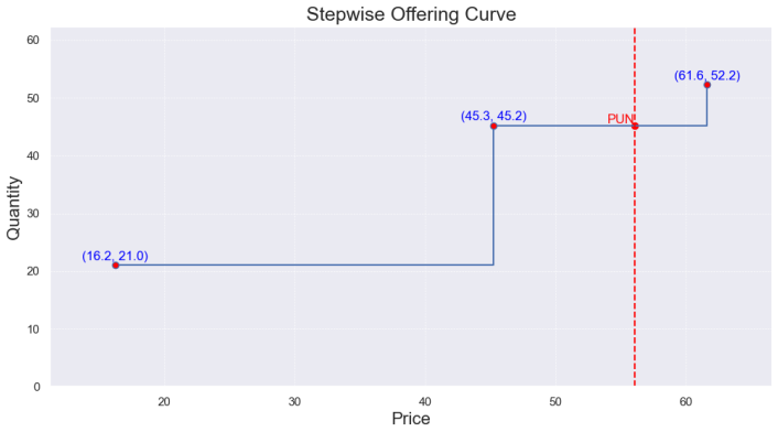
The workhorse is Deep Deterministic Policy Gradient with feed-forward actor and critic networks, soft-updated target networks, a replay buffer, and Ornstein-Uhlenbeck exploration noise. The action is a stepwise offering curve with three volume-price steps; the state is a 7-day batch of PUN prices; the reward is Eq. (7), which uses the indicator $\mathbf{1}_{\{P_i \le \mathrm{PUN}_{t+1}\}}$ to count accepted steps and subtracts production cost $C_k$ for each mode. The deterministic policy gradient update weaves the actor through the critic's Q-value gradient, which is the mechanism that lets the search run over a continuous action space.
What would settle it
Settle a held-out week of PUN prices twice for the trained policy: once with the paper's reward as printed, and once with each accepted volume allocated to the cheapest available mode up to its capacity $D_k$. If the two settlements rank alternative policies differently, or if the reported convergence disappears when the reward is corrected, the learning signal is an artifact of the summed reward rather than true profit.
Extended reading notes
Core claim
The central claim is that the deterministic policy gradient framework, adapted to a day-ahead electricity auction, converges to a useful offering policy in a fully observable environment whose state is a 168-dimensional matrix of hourly prices. The reward function in Eq. (7) pays the difference between offered revenue and production cost for every step whose price is at or below the next-day PUN, summed over the three production modes. The paper interprets the decreasing policy loss, the delayed decrease of the critic loss, and the increasing normalized reward as evidence that the agent is moving toward a more profitable strategy over time.
Load-bearing premise
The reward function used for training counts every accepted unit of volume as profit for all three production modes at once and never applies the stated capacity limits, so the number the agent maximizes may not be the seller's actual profit.
Editorial extensions
If this is right
- A seller can build an offering curve from a 7-day window of historical PUN prices without observing competitors' bids.
- The critic's Q-value estimate is unreliable early in training, so stable learning requires many episodes and slow target-network updates.
- An episode length below 15 days prevents convergence, while longer episodes improve exploration but show diminishing returns.
- The DDPG approach extends the earlier Q-learning supplier-bidding method to continuous action spaces by replacing discrete Q-tables with deep networks and a deterministic policy gradient.
- Because production costs and capacities are treated as fixed constants, the current model does not capture renewable intermittency; the paper proposes stochastic production as future work.
Reading between the lines
- A testable extension is to make production costs and capacities stochastic and feed current renewable output into the state; the authors mention this direction, and one would expect the agent to learn a hedging policy rather than a fixed mark-up.
- Because the environment treats PUN as an exogenous price process, the learned policy is a best response to history, not to adapting rivals; a multi-agent version with many similar sellers learning simultaneously, which the paper lists as future work, would test whether the strategy remains profitable when other sellers also learn.
- Reporting absolute profit in euros per episode alongside the normalized reward would let a reader judge economic significance; the paper currently gives only relative training metrics.
Editorial analysis
A structured set of objections, weighed in public.
Referee Report
Summary. The paper proposes a Deep Deterministic Policy Gradient (DDPG) agent that learns a stepwise offering curve for a seller in the Italian day-ahead electricity market. The state is a 7-day window of historical PUN prices, the action is an I-step price-volume curve, and the reward (Eq. (7)) is defined as the revenue from accepted bids minus production costs across K production modes. The authors train the agent on four years of hourly PUN data and report policy loss, critic loss, and a normalized reward during training, concluding that the agent learns to operate with greater efficiency and maximize payout.
Significance. The problem is practically relevant, and the use of DDPG for continuous-action bidding on real price data is a reasonable direction that could extend earlier Q-learning approaches. However, the current manuscript does not establish its central claim. The reward function in Eq. (7) is internally inconsistent as a model of profit, and the only reported evidence consists of training curves for that same misspecified objective. There is no baseline, no out-of-sample evaluation, and no test of whether the learned policy yields higher profit under a correct market settlement. The paper is transparent about its assumptions and limitations, which is a positive feature, but the numerical results do not support the headline conclusion as written.
major comments (3)
- [Sec. 2.2, Eq. (7)] The reward definition double-counts volume across production modes. For each accepted bid i, Eq. (7) sums (Pi*Vi - Ck*Vi) over all k=1..K, so each MWh is paid K times and charged with all K marginal costs. With the paper's values K=3, C=[10,30,60], one accepted bid at P=50, V=100 gives r=100*(3*50 - 100)=5000, whereas the largest feasible dispatch profit, respecting capacities D=[30,200,800] and allocating volume to the cheapest modes first, is (50-10)*30+(50-30)*70=2600. The DDPG agent therefore maximizes a fictitious payoff, not the realized profit described in the text, so the reported reward and loss curves are not evidence of profit-maximizing bidding.
- [Sec. 2.2 and Sec. 4.1] The capacity constraints D_k, set to [30,200,800] in Sec. 4.1, never enter the reward and never constrain the action. The actor network can propose volumes exceeding a mode's capacity and Eq. (7) rewards those volumes in full. A correct profit model must allocate each accepted bid's volume across production modes up to their capacities D_k, e.g., in merit order, and compute profit from the allocated volumes and each mode's cost. Without this, the learned policy has no relationship to the physical or economic constraints of the seller.
- [Sec. 4.2] The normalized reward is defined as r/rmax, where both r and rmax are computed from the same misspecified Eq. (7) and the same PUN series used for training. This makes the reported normalized reward circular as a performance metric. Furthermore, the only reported evidence is training dynamics: decreasing policy loss, decreasing critic loss after an initial spike, and increasing normalized reward. There is no baseline strategy (e.g., bid at marginal cost), no evaluation on a held-out time period, and no comparison of the learned policy's profit under a correct settlement. The abstract's claim that the participant gains the ability to maximize individual payout is therefore unsupported by the presented experiments.
minor comments (6)
- [Sec. 2.2, Fig. 5 caption] The caption says the reward is computed using accepted offers with 'offered price less than the registered pun', but Eq. (7) uses Pi <= PUN_{t+1}; the caption should say 'less than or equal to'.
- [Sec. 2.2, text near Eq. (7)] The sentence 'The curve of the Actor NN is obtained as the offering that minimizes the reward (in terms of obtained profit)' should read 'maximizes', since the agent optimizes expected cumulative reward.
- [Sec. 4.1] The notation C_i = [10, 30, 60] and D_i = [30, 200, 800] uses the step index i, while Section 2.2 uses i for bid steps and k for production modes. Please use C_k and D_k to avoid confusion.
- [Sec. 4.1] The sentence 'Another hypothesis we introduce is that the agent only knows about its expenses...' is an assumption, not a hypothesis; rephrase to 'We assume that the agent knows only its own expenses, available resources, and historical prices.'
- [Sec. 4.3] The sentence 'The first type consists of the action space’s partial observability...' reads awkwardly because the list that follows mixes market-design challenges and RL challenges; consider splitting into two explicit enumerations.
- [General] The paper does not mention whether code or trained agents will be released; providing reproducible code and the exact data preprocessing (e.g., timezone handling for PUN data) would strengthen future revisions.
Circularity Check
No significant circularity: the reward defines the objective, and the capacity/reward mismatch is a modeling-error concern, not a self-referential derivation.
full rationale
The paper follows a standard RL derivation chain: the state is historical PUN prices, the action is an offering curve, the reward is defined by Eq. (7), and DDPG updates the policy to maximize that reward. The abstract's claim that the participant maximizes individual payout is conditional on Eq. (7) actually representing realized profit; whether it does is a question of model correctness, not of circularity. The normalized reward is defined as r/rmax using the same r from Eq. (7), so training and evaluation share the same objective. This is definitional in any RL setup and does not amount to presenting a fitted parameter as an independent prediction. There is no load-bearing self-citation, no uniqueness theorem imported from the authors, and no ansatz smuggled in via citation. The paper does introduce capacities D_k and then never uses them in Eq. (7), which may make the reward misspecified relative to the stated physical constraints; however, that is an internal consistency error, not a circular step in which a claimed prediction reduces by construction to its input. Accordingly, the appropriate circularity score is 0.
Assumptions & free parameters
free parameters (7)
- Number of bid steps I =
3
- Production costs C_k =
[10, 30, 60] EUR/MWh
- Production capacities D_k =
[30, 200, 800]
- Ornstein-Uhlenbeck noise parameters =
theta=0.15, mu=1, sigma in [1,10]
- Episode length =
15, 20, or 30 days
- DDPG hyperparameter set =
Table 1 values
- State window length =
7 days (168 hourly PUN values)
assumptions (5)
- domain assumption EUPHEMIA clears the market at PUN and the single seller's bids do not affect that price.
- domain assumption The market is fully observable from historical PUN, production costs, and capacities.
- domain assumption Production costs and capacities are constant over the whole period.
- domain assumption Competitors' strategies are irrelevant to the agent's reward.
- domain assumption Using the realized next-day PUN in the reward is a valid training signal for a bidding decision made before PUN is known.
Cite this review
Pith. "Pith review of Reinforcement Learning for Bidding Strategy Optimization in Day-Ahead Energy Market." pith.science (2026). https://pith.science/paper/OBDDIAF7
@misc{pith2026241116519,
  author       = {Pith},
  title        = {Pith review of: Reinforcement Learning for Bidding Strategy Optimization in Day-Ahead Energy Market},
  year         = {2026},
  howpublished = {\url{https://pith.science/paper/OBDDIAF7}},
  note         = {Machine review of arXiv:2411.16519}
}
read the original abstract
In a day-ahead market, energy buyers and sellers submit their bids for a particular future time, including the amount of energy they wish to buy or sell and the price they are prepared to pay or receive. However, the dynamic for forming the Market Clearing Price (MCP) dictated by the bidding mechanism is frequently overlooked in the literature on energy market modelling. Forecasting models usually focus on predicting the MCP rather than trying to build the optimal supply and demand curves for a given price scenario. Following this approach, the article focuses on developing a bidding strategy for a seller in a continuous action space through a single agent Reinforcement Learning algorithm, specifically the Deep Deterministic Policy Gradient. The algorithm controls the offering curve (action) based on past data (state) to optimize future payoffs (rewards). The participant can access historical data on production costs, capacity, and prices for various sources, including renewable and fossil fuels. The participant gains the ability to operate in the market with greater efficiency over time to maximize individual payout.
Figures


Figures from the paper (10 more)



Reference graph
Works this paper leans on
-
[18]
Selecting and ranking individualized treatment rules with unmeasured confounding
Xiong, G., T. Hashiyama and S. Okuma, "An electricity supplier bidding strategy through Q-Learning,"IEEE Power Engineering Society Summer Meeting, pp. 1516-1521 vol.3, doi: 10.1109/PESS.2002.1043645 , (2002)
work page Pith review arXiv 2002
-
[19]
Deep Reinforcement Learning for Strategic Bidding in Electricity Markets,
Ye, Y., Qiu, D., Sun, M., Papadaskalopoulos D. and Strbac, G. "Deep Reinforcement Learning for Strategic Bidding in Electricity Markets," in IEEE Transactions on Smart Grid, vol. 11, no. 2, pp. 1343-1355, March 2020, doi: 10.1109/TSG.2019.2936142
arXiv 2020
-
[1]
Multiagent Rein- forcement Learning: A Review of Challenges and Applications
Canese, Lorenzo, Gian Carlo Cardarilli, Luca Di Nunzio, Rocco Fazzolari, Daniele Giardino, Marco Re, and Sergio Spanò. 2021. "Multiagent Rein- forcement Learning: A Review of Challenges and Applications" Applied Sciences 11, no. 11: 4948. https://doi.org/10.3390/app11114948
-
[2]
EUPHEMIA Public Description Single Price Coupling Algorithm (October 2020), available online from: https://www.nordpoolgroup. com/globalassets/download-center/single-day-ahead-coupling/ euphemia-public-description.pdf (2020) 23
work page 2020
- [3]
-
[4]
Multiagent deep reinforcement learning: a sur- vey
Gronauer, S., Diepold, K. Multiagent deep reinforcement learning: a sur- vey. Artif Intell Rev 55, 895–943 (2022). https://doi.org/10.1007/s10462- 021-09996-w
doi:10.1007/s10462- 2022
-
[5]
Reinforcement learning and stochastic optimization
Jaimungal, S. Reinforcement learning and stochastic optimization. Fi- nance Stoch 26, 103–129 (2022). https://doi.org/10.1007/s00780-021- 00467-2
-
[6]
Konda, V. R., & Tsitsiklis, J. N. (2000). Actor-critic algorithms. In Advances in Neural Information Processing Systems (pp. 1008-1014)
work page 2000
Show all 20 references
-
[7]
Optimization for Reinforcement Learning: From a single agent to cooperative agents,
Lee, D., He, N., Kamalaruban, P. and Cevher, V., "Optimization for Reinforcement Learning: From a single agent to cooperative agents," in IEEE Signal Processing Magazine, vol. 37, no. 3, pp. 123-135, May 2020, doi: 10.1109/MSP.2020.2976000
2020
-
[8]
Multiagent Reinforcement Learning in Sequential Social Dilemmas
Leibo, J. Z., Vinícius Flores Zambaldi, Marc Lanctot, Janusz Marecki and Thore Graepel. “Multiagent Reinforcement Learning in Sequential Social Dilemmas.” ArXiv abs/1702.03037 (2017): n. pag
2017 arXiv
-
[9]
Continuous control with deep reinforcement learning,
Lillicrap, T. P., Hunt, J. J., Pritzel, A., Heess, N., Erez, T. and Tassa, Y. “Continuous control with deep reinforcement learning,” Computer Science, vol. 8, no. 6, 2015
2015
-
[10]
Forecasting electricity prices, Oxford research encyclopedia of economics and finance
Maciejowska, K., B.Uniejewski, Weron, R., 2022. Forecasting electricity prices, Oxford research encyclopedia of economics and finance
2022
-
[11]
A., Veness, J., Bellemare, M
Mnih, V., Kavukcuoglu, K., Silver, D., Rusu, A. A., Veness, J., Bellemare, M. G., ... and Hassabis, D. (2015). Human-level control through deep reinforcement learning. Nature, 518(7540), 529-533
2015
-
[12]
Nicolaisen, T., Petrov, V., and Tesfatsion, L. (2001). Market power and efficiency in a computational electricity market with discriminatory double-auction pricing.IEEE Transactions on Evolutionary Computation, 5(5), 504-523. 24
2001
-
[13]
, Knapp, A
Posor, J.E., Belzner, L. , Knapp, A. Joint Action Learning for Multiagent Cooperation using Recurrent Reinforcement Learning. Digitale Welt 4, 79–84 (2020). https://doi.org/10.1007/s42354-019-0239-y
2020 doi
-
[14]
and Kebriaei, H
Rashedi, N., Tajeddini, M.A. and Kebriaei, H. (2016), Markov game approach for multiagent competitive bidding strategies in the electricity market. IET Gener. Transm. Distrib., 10: 3756-3763. https://doi.org/10.1049/iet-gtd.2016.0075
2016
-
[15]
Reinforcement Learning: An Introduction; MIT Press: Cambridge, MA, USA, 2018
Sutton, R.S.; Barto, A.G. Reinforcement Learning: An Introduction; MIT Press: Cambridge, MA, USA, 2018
2018
-
[16]
(2017) Multiagent cooperation and competition with deep reinforcement learning
Tampuu A, Matiisen T, Kodelja D, Kuzovkin I, Korjus K, Aru J, et al. (2017) Multiagent cooperation and competition with deep reinforcement learning. PLoS ONE 12(4): e0172395. https://doi.org/10.1371/journal.pone.0172395
2017 doi
-
[17]
J., & Dayan, P
Watkins, C. J., & Dayan, P. (1992). Q-learning.Machine learning, 8(3-4), 279-292
1992
-
[20]
PLoS ONE 9(7): e102840
Zou Y, Zhan W, Shao Y (2014) Evolution with Reinforce- ment Learning in Negotiation. PLoS ONE 9(7): e102840. https://doi.org/10.1371/journal.pone.0102840 25
2014 doi
Reviewed August 12, 2026 · model on record in the stance chip above.
Discussion (0). Continue with ORCID to comment.