REVIEW 3 major objections 4 minor 49 references
On forced swarmalators that move in higher-dimensional spaces
T0 review · 3 major / 4 minor · reviewed 2026-08-12 · deepseek-v4-flash
Pith's one-line read This paper derives the first analytical stability boundaries for forced swarmalators moving in two and three dimensions with periodic boundary conditions, giving exact curves for pinned, split-pinned, sync-dots, and phase-locked states.
desk verdict Useful extension of the 1D forced swarmalator analysis to 2D and 3D, but the advertised sync-dots stability boundary rests on an unproven slice ansatz and should be presented as numerical instead of analytic. read the letter →
The pith
A machine-rendered reading of the paper's core claim, the machinery that carries it, and where it could break.
The reading
What carries the argument
The technical workhorse is linear stability analysis at fixed points. For the pinned and split-pinned configurations, the Jacobian has a block structure that separates spatial and phase directions; its eigenvalues are computed exactly, and stability boundaries appear as zero-eigenvalue bifurcations, $F_c = -2K$ in 2D and $F_c = -3K$ in 3D. For sync dots and phase-locked states, the analysis reduces the swarmalator equations to fixed-point conditions such as $\cos\Delta x + \cos\Delta y = -\sqrt{2}F/K$, and the sync-dots stability boundary is obtained by setting one of the spatial separations ($\Delta y$ in 2D, two of the three in 3D) to zero, with the resulting condition asserted on numerical grounds to be the exact boundary for the full state.
What would settle it
Simulate Eq. (3) starting from two sync-dot clusters with both $\Delta x$ and $\Delta y$ nonzero and with unequal cluster sizes, slowly ramp $F$ at fixed $K<0$, and record the forcing values at which the two dots lose stability or the phase separation leaves $\theta^* = \pi/4$; if these values differ from Eq. (19) in 2D or Eq. (32) in 3D, the claimed exact boundary is falsified.
Extended reading notes
Core claim
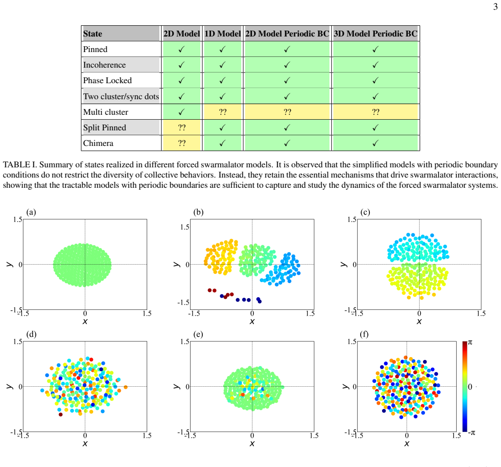
On its own terms, the paper's central claim is that a simplified forced swarmalator model on a periodic 2D torus, and its 3D analogue, reproduces the collective states of the full higher-dimensional model while remaining analytically tractable, and that the static states have computable stability boundaries. In 2D these are $F > -2K$ for the pinned state, $F < 2K$ for $K>0$ for split pinned, $-(2K+1)/\sqrt{2} < F < -2K/\sqrt{2}$ for sync dots, and $-2K/\sqrt{2} < F < -2K$ for phase locked, with the sync-dots and phase-locked bands requiring $K<0$. In 3D the same boundaries hold with $K$ replaced by $3K$ where it multiplies the spatial dimension, and the sync-dots band shifted accordingly. The paper also arranges the 1D, 2D, and 3D results in Table II, exposing a $p$-dimensional pattern $F > -pK$ for pinning, and reports numerical evidence that the periodic-boundary model reproduces the behavior of the power-law-kernel forced swarmalator model.
Load-bearing premise
The load-bearing premise is that the sync-dots stability boundary obtained by setting one spatial separation to zero, and then only checked numerically, is exactly the boundary of the full sync-dots state with both separations free.
Editorial extensions
If this is right
- The analytical curves in the $(K,F)$ plane, given by Eqs. (12), (16), (19), and (24) in 2D and their 3D analogues, give future numerical studies of forced swarmalators a precise set of bifurcation points to test.
- Table II's pattern suggests a general rule in $p$ spatial dimensions: pinning requires $F > -pK$, split pinning requires $F < pK$, and the sync-dots and phase-locked bands scale with $p$ as well.
- Because the periodic-boundary model omits hard-shell repulsion yet still produces all the collective states found in the full 2D forced model, it can serve as a minimal reliable model for forced swarmalator dynamics.
- The reported numerical agreement between the periodic-boundary model and the power-law-kernel model implies that analytically derived boundaries may transfer approximately to the more realistic model, giving predictions where only simulations existed before.
- The stability analysis also fixes where each static state loses stability as forcing strength $F$ is ramped upward, which directly describes how an external field can be tuned to pin or unlock a swarmalator population.
Reading between the lines
- The $p$-dimensional scaling visible in Table II is likely exact for all $p$, because the same block-Jacobian argument that gives $F=-2K$ in 2D and $F=-3K$ in 3D should give $F=-pK$ in general, so one could extend the analytic phase diagram to higher-dimensional tori by symmetry alone.
- If the sync-dots boundary is truly independent of the spatial separation pattern, it may also control the stability of the coherent sync-dot clusters observed inside the unanalysed chimera state, which would give a first analytical handle on that state.
- A direct numerical test of the special-case assumption is possible: integrate Eq. (3) with two sync-dot clusters separated in both $x$ and $y$, measure where the two dots lose stability, and compare with Eq. (19); a mismatch would show the claimed exactness is only approximate.
- The reported equivalence with the power-law-kernel model is presently numerical; a stronger version would use the periodic-boundary phase diagram to predict, for each $(K,F)$, which of the six states the full model exhibits and how hard-shell repulsion shifts the state boundaries.
Editorial analysis
A structured set of objections, weighed in public.
Referee Report
Summary. The paper studies forced swarmalator models in two and three spatial dimensions with periodic boundary conditions, extending a previously studied one-dimensional model. For the 2D and 3D models the authors derive analytic stability boundaries for four static collective states (pinned, split-pinned, sync dots, and phase locked) using linear stability analysis, and they support these boundaries with numerical phase diagrams. They also report that the simplified periodic-boundary models reproduce the collective states observed in a more realistic power-law swarmalator model, and they propose a p-dimensional extrapolation of the boundaries. The paper claims these are the first analytical results for forced swarmalators in two and three dimensions.
Significance. If the derived boundaries are correct, the paper makes a useful contribution by moving the analytic theory of forced swarmalators beyond one dimension and by identifying simple formulas that scale with the spatial dimension. The pinned and split-pinned analyses are clean, self-contained linear-stability derivations with no fitted parameters, and the numerical phase diagrams give concrete, testable predictions. The sync-dots and phase-locked boundaries, however, rest on an unproven reduction to a special submanifold of fixed points, so the central claim of exact analytical boundaries is not fully established as written. The paper is clearly organized and the numerical methodology is adequately documented, but the load-bearing analytical step for the sync-dots state needs either a rigorous justification or an explicit downgrade to a conjecture.
major comments (3)
- [Section IV.A.3, Eqs. (17)-(19)] The stability boundary for the sync dots state is derived by setting one of the two spatial separations to zero, Delta y = 0, and the text asserts that numerics suggests this slice provides the exact stability boundary for the full sync-dots state. The Jacobian at a generic sync-dots fixed point, however, depends on sin Delta x and sin Delta y separately: for example, the phase equation linearizes to terms proportional to (K/2) sin Delta x and (K/2) sin Delta y, and the position-phase coupling contains analogous factors, so the eigenvalues are not determined solely by cos Delta x + cos Delta y. No symmetry argument or coordinate transformation is supplied that makes the Delta y = 0 slice lossless. Because Eq. (19) is the advertised stability boundary for sync dots and also provides one endpoint of the phase-locked boundary Eq. (24), this unproven reduction is load-bearing. Please either prove that the stability condition is independent of the slice (e.g., by an explicit eigenvalue computation for the full fixed-point family) or explicitly state Eq. (19) as a numerically supported conjecture rather than an exact analytical result.
- [Section IV.B.3, Eqs. (30)-(32)] The same unproven reduction is used in the three-dimensional analysis, where two of the three spatial separations are set to zero before computing the eigenvalues of the sync-dots Jacobian. The resulting boundary Eq. (32) is presented as exact, and the phase-locked boundary Eq. (35) inherits this issue. In 3D the Jacobian at a generic sync-dots fixed point will contain coupling terms proportional to sin Delta x, sin Delta y, and sin Delta z, so the reduction is not obviously lossless. The claim that Eq. (32) is the exact stability boundary therefore needs the same kind of justification as in the 2D case; otherwise it should be labeled as a conjecture supported by the numerics shown in Fig. 8.
- [Section IV.A.3, paragraph after Eq. (17)] The derivation of the sync-dots eigenvalues assumes the population splits evenly between the two clusters, with the statement 'without loss of generality' and a further assertion that numerics indicate stability is independent of the population split. This is another unproven assumption in the sync-dots analysis. If the exact stability boundary really is independent of the cluster population split, this should be demonstrated analytically within the reduced model or, failing that, explicitly listed as part of the numerical conjecture.
minor comments (4)
- [Eq. (10) and Eq. (14)] In the Jacobian block M1 for the pinned state, the off-diagonal entry should be 2K/N rather than K/N, because at the pinned fixed point cos(x_j - x_i) + cos(y_j - y_i) = 2. As printed, the matrix is inconsistent with the stated eigenvalues -F and -F - 2K. The same factor-of-two issue appears in the off-diagonal entries of Eq. (14) for the split-pinned state. The eigenvalues listed in Eqs. (11) and (15) are consistent with the 2K/N off-diagonal, so I assume this is a typographical error, but it should be corrected.
- [Table II and Section V] The p-dimensional column of Table II is presented without derivation, and Section V says the framework 'allows us to predict analytical phase boundaries' in p dimensions. Since the formulas for p = 2 and p = 3 are themselves only conditionally established (see the sync-dots comments), the p-dimensional extrapolation should be explicitly labeled as conjectured, or a derivation should be supplied.
- [Abstract and Introduction] The claim that these are 'the first analytical results about swarmalator with forcing in two and three spatial dimensions' may overstate the scope, since the analysis applies to the periodic-boundary simplification rather than the original power-law model. I suggest wording such as 'first analytical stability results for the periodic-boundary forced swarmalator model in two and three dimensions'.
- [Throughout] There are several typographical errors: 'Notie' in the Table I caption, 'Varaition' in the Fig. 7 caption, 'Mspilt pinned' in Section IV.A.2, 'The details analysis' in Section II, and 'C()' where C_x, C_y are meant in Section IV.A.3. These should be corrected in a revision.
Circularity Check
No significant circularity: the stability boundaries are self-contained linear stability derivations; the Δy=0 sync-dots reduction is an unproven ansatz, not a circular step.
full rationale
The paper's analytic claims are self-contained stability calculations in the resonant frame with J=1. The pinned-state boundary (Eq. 12), split-pinned boundary (Eq. 16), sync-dots boundary (Eq. 19), and phase-locked boundary (Eq. 24) are all derived from explicit Jacobian eigenvalue computations or fixed-point conditions, with no fitted parameters and no quantity defined in terms of the predicted quantity. The only mathematically incomplete step is in Section IV.A.3, where the sync-dots fixed-point manifold cos Δx + cos Δy = -√2 F/K is reduced by setting Δy = 0, and the text says 'Numerics suggests that the acquired stability condition due to the consideration of these fixed points provides the exact stability boundary for the sync dots state.' This is an unsupported reduction and a numerical conjecture, but it is not circular in the sense of the target result being equivalent to its inputs by construction; it is a restriction of the fixed-point family followed by an external numerical check. The 3D sync-dots boundary (Eq. 32) inherits the same unproven reduction, again as an ansatz rather than a circular identity. Citations to the authors' prior 1D paper [36] for the eigenvalue procedure are method transfers, not load-bearing self-citations of the result itself, and [18] supplies the independent unforced-model results. No self-definitional, fitted-input-as-prediction, or self-citation-chain circularity is exhibited, so a non-finding with score 0 is appropriate.
Assumptions & free parameters
assumptions (5)
- domain assumption Resonant forcing with identical agents: natural frequencies set to zero and J=1 via rescaling.
- domain assumption The periodic-boundary model without hard-shell repulsion faithfully represents the original power-law kernel model.
- ad hoc to paper The sync-dots stability boundary from the Delta y=0 special case is exact.
- ad hoc to paper Stability of sync dots is independent of the cluster population split.
- ad hoc to paper The p-dimensional formulas in Table II are valid extrapolations.
Cite this review
Pith. "Pith review of On forced swarmalators that move in higher-dimensional spaces." pith.science (2026). https://pith.science/paper/ZLAKZJEZ
@misc{pith2026241117336,
  author       = {Pith},
  title        = {Pith review of: On forced swarmalators that move in higher-dimensional spaces},
  year         = {2026},
  howpublished = {\url{https://pith.science/paper/ZLAKZJEZ}},
  note         = {Machine review of arXiv:2411.17336}
}
read the original abstract
We study the collective dynamics of swarmalators subjected to periodic (sinusoidal) forcing. Although previous research focused on the simplified case of motion in a one-dimensional (1D) periodic domain, we extend this analysis to the more realistic scenario of motion in two and three spatial dimensions with periodic boundary conditions. In doing so, we identify analogues of the 1D states and characterize their dynamics and stability boundaries analytically. Additionally, we investigate the forced swarmalators model with power-law interaction kernels, finding that the analytically tractable model with periodic boundary conditions can reproduce the observed dynamic behaviors of this more complex model.
Figures


Figures from the paper (5 more)



Reference graph
Works this paper leans on
-
[1]
Analysis of pinned state In the pinned state, the fixed points are xi = Cx, yi = Cy, θi = 0 (7) for some constants Cx,Cy. The Jacobian Mpinned evaluated at this point has a simple block structure Mpinned = M0 0 0 0 M0 0 0 0 M1 , (8) where M0 and M1 are N × N blocks. Here, M0i j = − N − 1 N for i = j, 1 N for i ̸= j, (9) 8 FIG. 8. Phase...
-
[2]
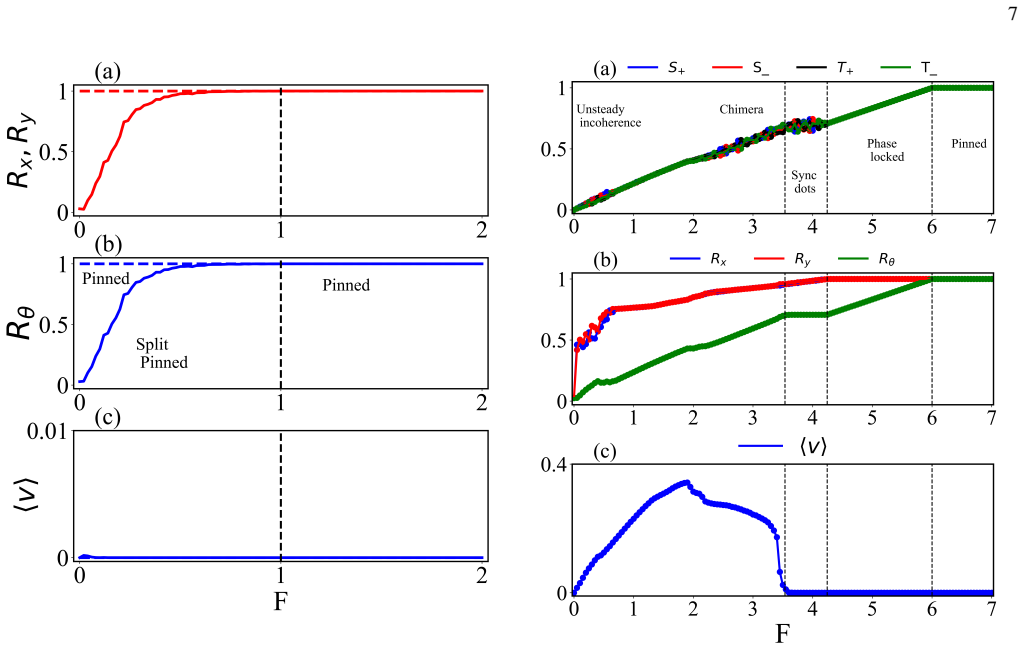
As F continues to grow, the sync dots state bifur- cates into a phase-locked state, whereS± = T± = Rθ < 1 while Rx = Ry = 1, indicating phase locking with spatial coherence. Finally, for sufficiently large F, this phase-locked state tran- sitions into the pinned state, where all coherence parameters reach their maximal values. C. 3D swarmalator model with...
-
[3]
Analysis of split pinned state Here, the swarmalators form two clusters with fixed point (x1, y1, θ1) = (Cx,Cy,0) and (x2, y2, θ2) = (Cx + π,Cy + π, π). The Jacobian evaluated at the fixed points has a block struc- ture similar to that of the pinned state, i.e., Mspilt pinned = M0 0 0 0 M0 0 0 0 M1 , (13) where M0 is given as previously by Eq....
-
[4]
Analysis of sync dots In the sync dots, swarmalators form two groups, and the number of swarmalators in each group depends on the ini- tial conditions. The first group is defined by (x1, y1, θ1) = (Cx,Cy.θ ∗), while the second is defined by(x2, y2, θ2) = (Cx + ∆x,Cy + ∆y, −θ ∗). The constant C() is arbitrary and stems from the rotational symmetry in the ˙...
-
[5]
Analysis of phase locked state The fixed points here take the form xi = Cx, yi = Cy, θi ∈ (−a, a), (20) where C() and a are constants. Plugging these expressions into the equation of motions (3) gives us 2KRθ sin (ψθ − θi) − F sin θi = 0, (21) Assuming ψθ = 0 without loss of generality, we have 2KRθ = −F. (22) The state bifurcates from the sync dots confi...
-
[6]
Thus, the phase-locked state bifurcates from the sync dots along the critical curve: F = −K √ 2, (23) which aligns with the previously derived stability boundary for the sync dots. The pinned state, defined by θi = 0 (imply- ing Rθ = 1), bifurcates from the phase locked state along the critical curve F = −2K, matching its stability boundary. Therefore, th...
-
[7]
Analysis of pinned state In the pinned state, the fixed points are xi = Cx, yi = Cy, zi = Cz, θi = 0 (25) for some constant C.. Proceeding similarly to the analysis of the 2D model, we can obtain the eigenvalues of Jacobian Mpinned evaluated at the fixed points as λ0 = 0, λ1 = −1, λ2 = −F, λ3 = −F − 3K, (26) with multiplicities 3, (3N − 3), 1, N − 1, resp...
-
[8]
Analysis of split pinned state Here, the swarmalators form two clusters with fixed point (x1, y1, z1, θ1) = (Cx,Cy,Cz,0) and (x2, y2, z2, θ2) = (Cx + π,Cy + π,Cz + π, π). The Jacobian evaluated at the fixed points has the eigenvalues λ0 = 0, λ1 = −1, λ2 = F − 3K, λ4 = −F − 3K, λ5,6 = 1 2 − 3K ± √ 4F2 + 9K2 , (28) with multiplicities 3, 3N −3, N 2 −1, N 2 ...
Show all 49 references
-
[9]
The first group is defined by (x1, y1, z1, θ1) = (Cx,Cy,Cz, θ ∗), while the second is defined 10 by (x2, y2, z2, θ2) = (Cx + ∆x,Cy + ∆y,Cz + ∆z, −θ ∗)
Analysis of sync dots Here, as in the 2D system, swarmalators form two groups, and the number of swarmalators in each group depends on the initial conditions. The first group is defined by (x1, y1, z1, θ1) = (Cx,Cy,Cz, θ ∗), while the second is defined 10 by (x2, y2, z2, θ2) =...
-
[10]
Plugging these expressions into the equation of motions (4) gives us 3KRθ sin (ψθ − θi) − F sin θi = 0
Analysis of phase locked state The fixed points here take the form xi = Cx, yi = Cy, zi = Cz, θi ∈ (−a, a), (33) where C() and a are constants. Plugging these expressions into the equation of motions (4) gives us 3KRθ sin (ψθ − θi) − F sin θi = 0. (34) Assuming ψθ = 0 without ...
-
[11]
Y . Yang, J. Elgeti, and G. Gompper, Physical Review E 78, 061903 (2008)
2008
-
[12]
Creppy, F
A. Creppy, F. Plouraboué, O. Praud, X. Druart, S. Cazin, H. Yu, and P. Degond, Journal of The Royal Society Interface 13, 20160575 (2016)
2016
-
[13]
Quillen, A
A. Quillen, A. Peshkov, E. Wright, and S. McGaffigan, Physical Review E 104, 014412 (2021)
2021
-
[14]
Quillen, A
A. Quillen, A. Peshkov, B. Chakrabarti, N. Skerrett, S. Mc- Gaffigan, and R. Zapiach, Physical Review E 106, 064401 (2022)
2022
-
[15]
Aihara, T
I. Aihara, T. Mizumoto, T. Otsuka, H. Awano, K. Nagira, H. G. Okuno, and K. Aihara, Scientific Reports 4, 3891 (2014)
2014
-
[16]
Hrabec, V
A. Hrabec, V . Kˇrižáková, S. Pizzini, J. Sampaio, A. Thiaville, S. Rohart, and J. V ogel, Physical Review Letters 120, 227204 11 State 1D Model (p=1) 2D Model Periodic BC (p=2) 3D Model Periodic BC (p=3) pD Model Periodic BC ?? Pinned F > −K F > −2K F > −3K F > −pK Split Pinn...
2018
-
[17]
C. D. Tsiairis and A. Aulehla, Cell 164, 656 (2016)
2016
-
[18]
Riedl, I
M. Riedl, I. Mayer, J. Merrin, M. Sixt, and B. Hof, Nature Com- munications 14, 5633 (2023)
2023
- [19]
- [20]
-
[21]
J. Yan, M. Bloom, S. C. Bae, E. Luijten, and S. Granick, Nature 491, 578 (2012)
2012
-
[22]
Zhang, A
B. Zhang, A. Sokolov, and A. Snezhko, Nature Communica- tions 11, 1 (2020)
2020
-
[23]
Barcis, M
A. Barcis, M. Barcis, and C. Bettstetter, in 2019 International Symposium on Multi-Robot and Multi-Agent Systems (MRS) (IEEE, 2019), pp. 98–104
2019
-
[24]
Barcis and C
A. Barcis and C. Bettstetter, IEEE Access 8, 218752 (2020)
2020
-
[25]
J. D. Monaco, G. M. Hwang, K. M. Schultz, and K. Zhang, Biological Cybernetics 114, 269 (2020)
2020
-
[26]
Tanaka, Physical Review Letters 99, 134103 (2007)
D. Tanaka, Physical Review Letters 99, 134103 (2007)
2007
-
[27]
K. P. O’Keeffe, H. Hong, and S. H. Strogatz, Nature Commu- nications 8, 1504 (2017)
2017
-
[28]
O’Keeffe, G
K. O’Keeffe, G. K. Sar, M. S. Anwar, J. U. Lizárraga, M. A. de Aguiar, and D. Ghosh, inProceedings A (The Royal Society, 2024), vol. 480, p. 20240448
2024
-
[29]
N. Blum, A. Li, K. O’Keeffe, and O. Kogan, Physical Review E 109, 014205 (2024)
2024
-
[30]
G. K. Sar, S. N. Chowdhury, M. Perc, and D. Ghosh, New Jour- nal of Physics 24, 043004 (2022)
2022
-
[31]
J. U. Lizárraga and M. A. de Aguiar, Physical Review E 108, 024212 (2023)
2023
-
[32]
G. K. Sar, D. Ghosh, and K. O’Keeffe, Physical Review E 107, 024215 (2023)
2023
-
[33]
G. K. Sar, K. O’Keeffe, and D. Ghosh, Chaos: An Interdisci- plinary Journal of Nonlinear Science 33, 111103 (2023)
2023
-
[34]
G. K. Sar, D. Ghosh, and K. O’Keeffe, Physical Review E 109, 044603 (2024)
2024
-
[35]
H. Hong, K. P. O’Keeffe, J. S. Lee, and H. Park, Physical Re- view Research 5, 023105 (2023)
2023
-
[36]
S. Yoon, K. O’Keeffe, J. Mendes, and A. Goltsev, Physical Re- view Letters 129, 208002 (2022)
2022
-
[37]
M. S. Anwar, G. K. Sar, M. Perc, and D. Ghosh, Communica- tions Physics 7, 59 (2024)
2024
-
[38]
M. Urso, M. Ussia, and M. Pumera, Advanced Functional Ma- terials 31, 2101510 (2021)
2021
-
[39]
J. Dai, X. Cheng, X. Li, Z. Wang, Y . Wang, J. Zheng, J. Liu, J. Chen, C. Wu, and J. Tang, Advanced Functional Materials 31, 2106204 (2021)
2021
-
[40]
Vikrant and K.-H
K. Vikrant and K.-H. Kim, Catalysis Science & Technology (2021)
2021
-
[41]
Tesaˇr, M
J. Tesaˇr, M. Ussia, O. Alduhaish, and M. Pumera, Applied Ma- terials Today 26, 101312 (2022)
2022
-
[42]
J. Li, O. E. Shklyaev, T. Li, W. Liu, H. Shum, I. Rozen, A. C. Balazs, and J. Wang, Nano Letters 15, 7077 (2015)
2015
-
[43]
Cheng, W
R. Cheng, W. Huang, L. Huang, B. Yang, L. Mao, K. Jin, Q. ZhuGe, and Y . Zhao, ACS nano8, 7746 (2014)
2014
-
[44]
Manamanchaiyaporn, X
L. Manamanchaiyaporn, X. Tang, Y . Zheng, and X. Yan, IEEE Robotics and Automation Letters 6, 5605 (2021)
2021
-
[45]
Note1, see the Introduction in [18] for a discussion about the analytic difficulties of the 2D model
-
[46]
M. S. Anwar, D. Ghosh, and K. O’Keeffe, Physical Review E 110, 054205 (2024)
2024
-
[47]
O’Keeffe, S
K. O’Keeffe, S. Ceron, and K. Petersen, Physical Review E105, 014211 (2022)
2022
-
[48]
K. P. O’Keeffe, arXiv:2410.18011 (2024)
2024 arXiv
- [49]
Reviewed August 12, 2026 · model on record in the stance chip above.
Discussion (0). Continue with ORCID to comment.