REVIEW 4 major objections 6 minor 36 references
MFF-FTNet: Multi-scale Feature Fusion across Frequency and Temporal Domains for Time Series Forecasting
T0 review · 4 major / 6 minor · reviewed 2026-08-12 · deepseek-v4-flash
Pith's one-line read MFF-FTNet claims a 7.7% MSE win by fusing frequency and temporal contrastive features.
desk verdict A plausible combination of known components, but the paper never specifies how representations become forecasts, so the headline MSE gains are not reproducible from the text. read the letter →
The pith
A machine-rendered reading of the paper's core claim, the machinery that carries it, and where it could break.
The reading
What carries the argument
The load-bearing machinery is the pair of contrastive modules. The Frequency-Aware Contrastive Module transforms the latent representation with FFT, keeps the top-k amplitude frequencies (masking ratio $\alpha_m$), applies learnable weights and bias, returns via iFFT, and then computes separate contrastive losses on the amplitude and phase vectors ($L_{amp}$ and $L_{phase}$, combined as $L_{freq} = \lambda L_{amp} + (1-\lambda) L_{phase}$). The Complementary Time Domain Contrastive Module runs eight parallel 1D convolutions with kernel sizes [1,2,4,8,16,32,64,128], stacks the outputs, fuses them with 2D convolution and average pooling, and computes a time contrastive loss $L_{time}$ between the backbone output $r$ and the fused representation $h$. The total training loss is $L_{total} = \gamma_1 L_{time} + \gamma_2 L_{freq}$; these two losses are what the learning objective actually contains, and the reported forecasting performance is attributed to their combination.
What would settle it
Implement the training loop exactly as described with only the contrastive losses and check whether the trained model can output a forecast for any horizon; if the stated equations are the whole procedure, there is no mechanism to produce the prediction window, so the MSE numbers in the tables must come from an additional, undocumented component. Reproducing the tables only after adding an explicit forecasting head would settle the question.
Extended reading notes
Core claim
The central discovery, on the paper's own terms, is that splitting contrastive learning by frequency amplitude and phase, and simultaneously aligning the backbone representation with a fused multi-scale temporal representation, yields forecasting representations that beat existing contrastive and transformer baselines on every tested horizon. The authors attribute the gain to the frequency masking operation, which discards low-amplitude (mostly noisy) frequency bins, and to the multi-scale fusion, which lets the model see both short spikes and long trends at once. The reported numbers show the full model outperforming the strongest baseline by 7.7% average MSE on multivariate ETT datasets and 2.5% on univariate tasks across all five datasets. As stated, the improvement follows from the complementary domain alignment rather than from a new prediction head.
Load-bearing premise
The reported forecasting accuracy rests on the unstated assumption that a prediction step exists beyond the two contrastive losses, because the paper defines the total loss as $\gamma_1 L_{time} + \gamma_2 L_{freq}$ and never specifies the mapping $g(\cdot)$ that turns the learned representation into future values.
Editorial extensions
If this is right
- If the claimed 7.7% multivariate MSE gain holds, frequency-domain contrastive learning combined with multi-scale temporal fusion is a practical alternative to transformer-based forecasters on electricity and weather data.
- The robustness experiments imply that the learned representation is insensitive to up to 40% missing training data, which would make the approach attractive for real-world sensor streams with dropouts.
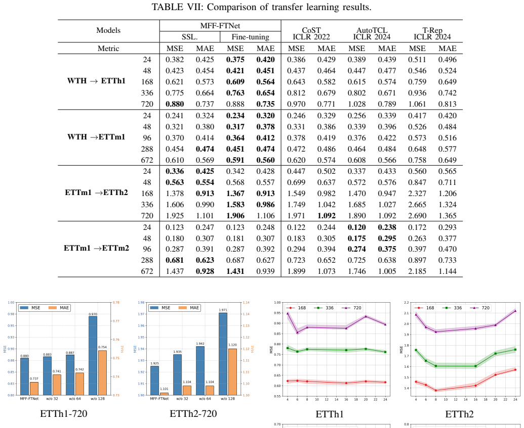
- The transfer-learning results imply that representations pretrained on one dataset (e.g., weather) can be fine-tuned effectively on another (e.g., ETT), reducing the need for large labeled forecasting datasets.
- The ablation ordering suggests that the multi-scale time-domain module contributes more than the frequency module on the tested datasets, which would guide future designs toward wider kernel banks.
Reading between the lines
- Because the paper specifies no forecasting head and no supervised loss, a reader cannot tell from the text alone how the final predictions are produced; the most natural reading is that an undocumented linear projection or fine-tuning step maps the representation to future values.
- A direct extension would be to make that step explicit by training a linear forecaster on top of the frozen contrastive representation; the paper's claims imply this linear probe should reproduce most of the reported accuracy.
- The two-module design is modular: the same frequency-aware and time-domain contrastive modules could be attached to other backbones for tasks like anomaly detection or classification, though the paper only evaluates forecasting.
- The reported noise-robustness suggests that top-k frequency masking is effectively a learned denoiser, which might be used as a preprocessing layer in other models rather than only inside a contrastive objective.
Editorial analysis
A structured set of objections, weighed in public.
Referee Report
Summary. The paper proposes MFF-FTNet, a time-series forecasting architecture combining an adaptive noise augmentation scheme, a Frequency-Aware Contrastive Module (FACM) that operates on FFT spectra with frequency masking and a dual contrastive loss, and a Complementary Time Domain Contrastive Module (CTCM) with multi-scale convolutions and feature fusion. The authors report state-of-the-art results on five datasets, claiming a 7.7% average MSE improvement over baselines in multivariate forecasting and a 2.5% improvement in univariate forecasting, plus ablation, robustness, transfer, and visualization experiments. The central problem is that the manuscript never specifies a forecasting head or any supervised prediction objective; the only training losses defined (Section III-G, Eq. 16) are contrastive losses, so the reported forecasting numbers cannot be reproduced from the described method. Several internal inconsistencies in the FACM equations and in the contrastive loss definitions compound this issue.
Significance. If the framework were fully specified and the empirical claims verified, the idea of combining frequency-selective contrastive learning with multi-scale temporal convolutions could be of interest to the time-series forecasting community. However, the paper as written does not provide a reproducible forecasting method: the prediction mechanism is absent, and the reported experimental results therefore do not establish the claimed improvements. The paper also presents no code, no detailed training procedure for the forecasting output, and the experimental comparison tables contain direct counterexamples to the 'consistently outperforms' claim. The contribution is thus currently not assessable as a forecasting method.
major comments (4)
- [Section III-G / Eq. (16)] The paper never defines a forecasting loss or a prediction head. Equation (16) defines L_total = γ1 L_time + γ2 L_freq, where L_time (Eq. 15) and L_freq (Eq. 10) are contrastive objectives, and neither term involves the future values XO or any supervised prediction error. Section III-A states that the goal is to learn g(·) with XO = g(X), but g is never specified, and no decoder, linear probe, or forecasting layer is described anywhere in Section III or Section IV. Consequently, the MSE and MAE numbers in Tables IV and V cannot be produced from the method as written, and a reader cannot reimplement the reported system.
- [Section III-E, Eqs. (4)–(6) and Algorithm 1] The FACM equations are dimensionally inconsistent. The input is r ∈ R^{T×K}, so its FFT should be a complex tensor of size T×K (or c×K after truncation), and averaging over the K dimension yields a vector of length T, not D. Yet Eq. (5) declares F ∈ R^{c×D}, and Algorithm 1 in Step 2 creates weights ωp ∈ R^{D×K/2} and biases βp ∈ R^{c×K/2}, mixing the latent dimension K with the input dimension D. This makes Equations (4)–(7) ill-defined as written; the authors must clarify the actual shapes used in their implementation.
- [Section III-E3, Eqs. (8)–(9)] The contrastive loss formulas do not match the accompanying text. The text states that 'different samples within the same batch are considered negative pairs,' but the denominators in Eqs. (8) and (9) sum over frequency indices k (k ≠ j) within the same pair of augmented views, not over other batch samples. Thus the equations define a loss that treats different frequency components as negatives, which is a different objective from the described batch-level contrastive learning. This discrepancy makes it impossible to determine what loss was actually minimized during training.
- [Section IV-D, Tables IV and V] The claim that MFF-FTNet 'consistently outperforms' baselines is contradicted by the reported numbers. In Table IV, on WTH with horizon 720, MFF-FTNet has MSE 0.534 while TCN achieves 0.498. In Table V, on ETTh2 with horizon 720, MFF-FTNet has MSE 0.212 versus TCN's 0.200, and on WTH horizons 168, 336, and 720, TCN and CoST surpass MFF-FTNet. Table VII also shows that on WTH→ETTh1 with horizon 24, CoST achieves 0.375 versus MFF-FTNet's 0.382. The aggregated percentage improvements in the text (7.7%, 2.5%) therefore do not reflect a consistent advantage, and the central claim needs to be substantially qualified.
minor comments (6)
- [Section III-C, Eq. (1)] The mean and standard deviation are written as functions of xt for t = 1,...,T, but xt is previously defined as a slice of X at time t with all D features; the notation should make clear whether the mean and variance are computed per feature dimension or as scalars.
- [Section IV-A and Table II] The text states that the Weather dataset contains 11 features, while Table II lists 12 features. Please reconcile this discrepancy.
- [Section IV-D, text after Table V] The paper claims an 8.9% MSE reduction on the ETT datasets compared to CoST, but it is not clear whether this figure is the average over the four ETT datasets or computed in some other way; the averaging procedure should be stated explicitly.
- [Figure 1] The figure is referenced in the abstract and introduction but appears to be a qualitative performance comparison without a caption or axis labels in the manuscript text; it should be described and referenced properly.
- [Section IV-E, Table VI] The ablation table reports a single MSE/MAE value for each variant without specifying the prediction horizon or whether the numbers are averaged over the horizons shown in the main tables; the experimental protocol for these ablations should be documented.
- [Section IV-G, Figures 7 and 8] The sensitivity analysis plots show performance trends but no numerical values or error bars; specifying the reported metric and the evaluation protocol would strengthen the claims about the effect of L′ and D′.
Circularity Check
No circularity found: the missing forecasting objective is an incompleteness/reproducibility issue, not a self-referential reduction.
full rationale
No circular step can be exhibited from the paper's equations or citations. The training objective in Eq. 16 is L_total = gamma1 * L_time + gamma2 * L_freq, where both terms are contrastive losses over representations derived from the same input; the forecasting map g(.) in Section III-A is never specified, and no prediction head or supervised forecasting loss is defined. That is a serious reproducibility and soundness gap, but it is not circularity: the reported MSE improvements do not reduce to a fitted parameter renamed as a prediction, nor does any equation define X in terms of Y or vice versa. The model borrows its backbone from CoST [21], frequency selection ideas from TimesNet [31], and contrastive formulations from TS2Vec/CoST, but these are external prior works, not self-citations by the present authors, and none is invoked as a uniqueness theorem to force the central claim. Hyperparameters are tuned on the same datasets where performance is reported, which is standard empirical practice rather than a self-referential derivation. Therefore the central claim rests on an underspecified experimental pipeline, not on a circular chain of reasoning, and the appropriate circularity score is 0.
Assumptions & free parameters
free parameters (6)
- α (noise scaling strength) =
not reported
- β (noise offset strength) =
not reported
- αm (frequency masking ratio) =
not reported
- λ (amplitude/phase balance) =
not reported
- γ1, γ2 (loss weights) =
not reported
- Convolution kernel sizes (n=8, kernels [1,2,4,8,16,32,64,128]) =
n=8, list as given
assumptions (3)
- domain assumption The contrastive representation learned by Ltime and Lfreq is sufficient for forecasting, since no forecasting loss is included in Ltotal.
- ad hoc to paper The FFT of r ∈ R^{T×K} can be represented as F ∈ R^{c×D}, mixing the latent dimension K with the input dimension D.
- domain assumption The baselines are evaluated under the same forecasting protocol as MFF-FTNet, including how representation models like TS2Vec and TNC are adapted to forecasting.
Cite this review
Pith. "Pith review of MFF-FTNet: Multi-scale Feature Fusion across Frequency and Temporal Domains for Time Series Forecasting." pith.science (2026). https://pith.science/paper/RRZ2JNOT
@misc{pith2026241117382,
  author       = {Pith},
  title        = {Pith review of: MFF-FTNet: Multi-scale Feature Fusion across Frequency and Temporal Domains for Time Series Forecasting},
  year         = {2026},
  howpublished = {\url{https://pith.science/paper/RRZ2JNOT}},
  note         = {Machine review of arXiv:2411.17382}
}
read the original abstract
Time series forecasting is crucial in many fields, yet current deep learning models struggle with noise, data sparsity, and capturing complex multi-scale patterns. This paper presents MFF-FTNet, a novel framework addressing these challenges by combining contrastive learning with multi-scale feature extraction across both frequency and time domains. MFF-FTNet introduces an adaptive noise augmentation strategy that adjusts scaling and shifting factors based on the statistical properties of the original time series data, enhancing model resilience to noise. The architecture is built around two complementary modules: a Frequency-Aware Contrastive Module (FACM) that refines spectral representations through frequency selection and contrastive learning, and a Complementary Time Domain Contrastive Module (CTCM) that captures both short- and long-term dependencies using multi-scale convolutions and feature fusion. A unified feature representation strategy enables robust contrastive learning across domains, creating an enriched framework for accurate forecasting. Extensive experiments on five real-world datasets demonstrate that MFF-FTNet significantly outperforms state-of-the-art models, achieving a 7.7% MSE improvement on multivariate tasks. These findings underscore MFF-FTNet's effectiveness in modeling complex temporal patterns and managing noise and sparsity, providing a comprehensive solution for both long- and short-term forecasting.
Figures


Figures from the paper (8 more)




Reference graph
Works this paper leans on
-
[1]
Doubleadapt: A meta-learning approach to incremental learning for stock trend forecasting,
L. Zhao, S. Kong, and Y . Shen, “Doubleadapt: A meta-learning approach to incremental learning for stock trend forecasting,” in Proceedings of the 29th ACM SIGKDD Conference on Knowledge Discovery and Data Mining, 2023, pp. 3492–3503
work page 2023
-
[2]
Ai in finance: challenges, techniques, and opportunities,
L. Cao, “Ai in finance: challenges, techniques, and opportunities,” ACM Computing Surveys (CSUR) , vol. 55, no. 3, pp. 1–38, 2022
work page 2022
-
[3]
An efficient equilibrium optimizer with support vector regression for stock market prediction,
E. H. Houssein, M. Dirar, L. Abualigah, and W. M. Mohamed, “An efficient equilibrium optimizer with support vector regression for stock market prediction,” Neural computing and applications, pp. 1–36, 2022
work page 2022
-
[4]
Accurate medium-range global weather forecasting with 3d neural networks,
K. Bi, L. Xie, H. Zhang, X. Chen, X. Gu, and Q. Tian, “Accurate medium-range global weather forecasting with 3d neural networks,” Nature, vol. 619, no. 7970, pp. 533–538, 2023
2023
-
[5]
D. Zhuang, V . J. Gan, Z. D. Tekler, A. Chong, S. Tian, and X. Shi, “Data-driven predictive control for smart hvac system in iot-integrated buildings with time-series forecasting and reinforcement learning,” Ap- plied Energy, vol. 338, p. 120936, 2023
work page 2023
-
[6]
Spatio-temporal meta-graph learning for traffic forecasting,
R. Jiang, Z. Wang, J. Yong, P. Jeph, Q. Chen, Y . Kobayashi, X. Song, S. Fukushima, and T. Suzumura, “Spatio-temporal meta-graph learning for traffic forecasting,” in Proceedings of the AAAI conference on artificial intelligence, vol. 37, no. 7, 2023, pp. 8078–8086
2023
-
[7]
Time series prediction using deep learning methods in healthcare,
M. A. Morid, O. R. L. Sheng, and J. Dunbar, “Time series prediction using deep learning methods in healthcare,” ACM Transactions on Management Information Systems , vol. 14, no. 1, pp. 1–29, 2023
work page 2023
-
[8]
Std: a seasonal-trend-dispersion decomposition of time se- ries,
G. Dudek, “Std: a seasonal-trend-dispersion decomposition of time se- ries,” IEEE Transactions on Knowledge and Data Engineering , vol. 35, no. 10, pp. 10 339–10 350, 2023
work page 2023
Show all 36 references
-
[9]
A rnn based time series approach for fore- casting turkish electricity load,
A. Tokg ¨oz and G. ¨Unal, “A rnn based time series approach for fore- casting turkish electricity load,” in 2018 26th Signal processing and communications applications conference (SIU) . IEEE, 2018, pp. 1–4
2018
-
[10]
Ngcu: A new rnn model for time-series data prediction,
J. Wang, X. Li, J. Li, Q. Sun, and H. Wang, “Ngcu: A new rnn model for time-series data prediction,” Big Data Research, vol. 27, p. 100296, 2022
2022
-
[11]
The performance of lstm and bilstm in forecasting time series,
S. Siami-Namini, N. Tavakoli, and A. S. Namin, “The performance of lstm and bilstm in forecasting time series,” in 2019 IEEE International conference on big data (Big Data) . IEEE, 2019, pp. 3285–3292
2019
-
[12]
U- net-lstm: time series-enhanced lake boundary prediction model,
L. Yin, L. Wang, T. Li, S. Lu, J. Tian, Z. Yin, X. Li, and W. Zheng, “U- net-lstm: time series-enhanced lake boundary prediction model,” Land, vol. 12, no. 10, p. 1859, 2023
2023
-
[13]
A cnn–lstm model for gold price time-series forecasting,
I. E. Livieris, E. Pintelas, and P. Pintelas, “A cnn–lstm model for gold price time-series forecasting,” Neural computing and applications , vol. 32, pp. 17 351–17 360, 2020
2020
-
[14]
Prediction for time series with cnn and lstm,
X. Jin, X. Yu, X. Wang, Y . Bai, T. Su, and J. Kong, “Prediction for time series with cnn and lstm,” in Proceedings of the 11th international con- ference on modelling, identification and control (ICMIC2019). Springer, 2020, pp. 631–641
2020
-
[15]
Ts2vec: Towards universal representation of time series,
Z. Yue, Y . Wang, J. Duan, T. Yang, C. Huang, Y . Tong, and B. Xu, “Ts2vec: Towards universal representation of time series,” in Proceed- ings of the AAAI Conference on Artificial Intelligence , vol. 36, no. 8, 2022, pp. 8980–8987
2022
-
[16]
T-rep: Representa- tion learning for time series using time-embeddings,
A. Fraikin, A. Bennetot, and S. Allassonni `ere, “T-rep: Representa- tion learning for time series using time-embeddings,” arXiv preprint arXiv:2310.04486, 2023
2023 arXiv
-
[17]
Simts: rethinking contrastive representation learning for time series forecasting,
X. Zheng, X. Chen, M. Sch ¨urch, A. Mollaysa, A. Allam, and M. Krauthammer, “Simts: rethinking contrastive representation learning for time series forecasting,” arXiv preprint arXiv:2303.18205 , 2023
2023 arXiv
-
[18]
Informer: Beyond efficient transformer for long sequence time-series forecasting,
H. Zhou, S. Zhang, J. Peng, S. Zhang, J. Li, H. Xiong, and W. Zhang, “Informer: Beyond efficient transformer for long sequence time-series forecasting,” in Proceedings of the AAAI conference on artificial intel- ligence, vol. 35, no. 12, 2021, pp. 11 106–11 115
2021
-
[19]
A time series is worth 64 words: Long-term forecasting with transformers,
Y . Nie, N. H. Nguyen, P. Sinthong, and J. Kalagnanam, “A time series is worth 64 words: Long-term forecasting with transformers,” arXiv preprint arXiv:2211.14730, 2022
2022 arXiv
-
[20]
Carla: Self-supervised contrastive representation learning for time se- ries anomaly detection,
Z. Z. Darban, G. I. Webb, S. Pan, C. C. Aggarwal, and M. Salehi, “Carla: Self-supervised contrastive representation learning for time se- ries anomaly detection,” Pattern Recognition, vol. 157, p. 110874, 2025
2025
-
[21]
Cost: Contrastive learning of disentangled seasonal-trend representations for time series forecasting,
G. Woo, C. Liu, D. Sahoo, A. Kumar, and S. Hoi, “Cost: Contrastive learning of disentangled seasonal-trend representations for time series forecasting,” arXiv preprint arXiv:2202.01575 , 2022
2022 arXiv
-
[22]
Fouriergnn: Rethinking multivariate time series forecast- ing from a pure graph perspective,
K. Yi, Q. Zhang, W. Fan, H. He, L. Hu, P. Wang, N. An, L. Cao, and Z. Niu, “Fouriergnn: Rethinking multivariate time series forecast- ing from a pure graph perspective,” Advances in Neural Information Processing Systems, vol. 36, 2024
2024
-
[23]
Crossgnn: Confronting noisy multivariate time series via cross interaction refinement,
Q. Huang, L. Shen, R. Zhang, S. Ding, B. Wang, Z. Zhou, and Y . Wang, “Crossgnn: Confronting noisy multivariate time series via cross interaction refinement,” Advances in Neural Information Processing Systems, vol. 36, pp. 46 885–46 902, 2023
2023
-
[24]
Crossformer: Transformer utilizing cross- dimension dependency for multivariate time series forecasting,
Y . Zhang and J. Yan, “Crossformer: Transformer utilizing cross- dimension dependency for multivariate time series forecasting,” in The eleventh international conference on learning representations , 2023
2023
-
[25]
A simple framework for contrastive learning of visual representations,
T. Chen, S. Kornblith, M. Norouzi, and G. Hinton, “A simple framework for contrastive learning of visual representations,” in International conference on machine learning . PMLR, 2020, pp. 1597–1607
2020
-
[26]
Unsupervised data augmentation for consistency training,
Q. Xie, Z. Dai, E. Hovy, T. Luong, and Q. Le, “Unsupervised data augmentation for consistency training,” Advances in neural information processing systems, vol. 33, pp. 6256–6268, 2020
2020
-
[27]
Graph con- trastive learning with augmentations,
Y . You, T. Chen, Y . Sui, T. Chen, Z. Wang, and Y . Shen, “Graph con- trastive learning with augmentations,” Advances in neural information processing systems, vol. 33, pp. 5812–5823, 2020
2020
-
[28]
Momentum contrast for unsupervised visual representation learning,
K. He, H. Fan, Y . Wu, S. Xie, and R. Girshick, “Momentum contrast for unsupervised visual representation learning,” in Proceedings of the IEEE/CVF conference on computer vision and pattern recognition, 2020, pp. 9729–9738
2020
-
[29]
Time-series representation learning via temporal and contextual con- trasting,
E. Eldele, M. Ragab, Z. Chen, M. Wu, C. K. Kwoh, X. Li, and C. Guan, “Time-series representation learning via temporal and contextual con- trasting,” arXiv preprint arXiv:2106.14112 , 2021
2021 arXiv
-
[30]
Timesurl: Self-supervised contrastive learning for universal time series representation learning,
J. Liu and S. Chen, “Timesurl: Self-supervised contrastive learning for universal time series representation learning,” in Proceedings of the AAAI Conference on Artificial Intelligence , vol. 38, no. 12, 2024, pp. 13 918–13 926
2024
-
[31]
Timesnet: Temporal 2d-variation modeling for general time series analysis,
H. Wu, T. Hu, Y . Liu, H. Zhou, J. Wang, and M. Long, “Timesnet: Temporal 2d-variation modeling for general time series analysis,” in The Eleventh International Conference on Learning Representations, ICLR 2023, Kigali, Rwanda, May 1-5, 2023 , 2023
2023
-
[32]
Periodicity decoupling framework for long-term series forecasting,
T. Dai, B. Wu, P. Liu, N. Li, J. Bao, Y . Jiang, and S.-T. Xia, “Periodicity decoupling framework for long-term series forecasting,” in The Twelfth International Conference on Learning Representations , 2024
2024
-
[33]
Tslanet: Rethinking transformers for time series representation learning,
E. Eldele, M. Ragab, Z. Chen, M. Wu, and X. Li, “Tslanet: Rethinking transformers for time series representation learning,” arXiv preprint arXiv:2404.08472, 2024
2024 arXiv
-
[34]
Unsupervised representa- tion learning for time series with temporal neighborhood coding,
S. Tonekaboni, D. Eytan, and A. Goldenberg, “Unsupervised representa- tion learning for time series with temporal neighborhood coding,” arXiv preprint arXiv:2106.00750, 2021
2021 arXiv
-
[35]
An empirical evaluation of generic convolutional and recurrent networks for sequence modeling,
S. Bai, J. Z. Kolter, and V . Koltun, “An empirical evaluation of generic convolutional and recurrent networks for sequence modeling,” arXiv preprint arXiv:1803.01271, 2018
2018 arXiv
-
[36]
Parametric augmentation for time series contrastive learning,
X. Zheng, T. Wang, W. Cheng, A. Ma, H. Chen, M. Sha, and D. Luo, “Parametric augmentation for time series contrastive learning,” arXiv preprint arXiv:2402.10434, 2024
2024 arXiv
Reviewed August 12, 2026 · model on record in the stance chip above.
Discussion (0). Continue with ORCID to comment.