REVIEW 3 major objections 4 minor 41 references
Kinetic Field Theory Applied to Planetesimal Formation I: Freely Streaming Dust Particles
T0 review · 3 major / 4 minor · reviewed 2026-08-12 · deepseek-v4-flash
Pith's one-line read Freely streaming dust inevitably develops a universal $k^{-3}$ density power-law tail at small scales.
desk verdict Useful KFT-for-planetesimals groundwork, but the universal k^-3 tail is not proven as cleanly as the paper claims. read the letter →
The pith
A machine-rendered reading of the paper's core claim, the machinery that carries it, and where it could break.
The reading
What carries the argument
The generating functional $Z$ of kinetic field theory, which integrates the initial phase-space probability distribution weighted by particle trajectories, together with the free-particle Green's function $G(t,t')$ (Hamiltonian $H=p^2/2m$, so that positions stream as $\bar q(t)=q_i+(t/m)p_i$). The power spectrum is extracted by applying two density operators to $Z$, and the small-scale asymptote is fixed by a saddle-point theorem for integrals of the form $\int e^{-|k|^s f(x)} g(x) e^{i k\cdot x}$, applied to the momentum-correlation shaping function $f(r)$ whose Hessian at the origin is positive definite. The momentum covariance matrix $\bar C_{pp}$, built from Gaussianized squared-density and momentum fields of a streaming-instability snapshot, supplies the initial correlations that make the tail universal.
What would settle it
Include a linear drag force with Stokes number $\mathrm{St}=0.01$ in the kinetic field theory equation of motion and recompute the small-scale asymptote; if the power spectrum slope changes from $k^{-3}$, the free-streaming result does not carry over to realistic streaming-instability conditions. A direct numerical check would be to measure the density power spectrum of a streaming-instability simulation at wave numbers $k\gtrsim 85$ at early times and test whether the slope is $-3$.
Extended reading notes
Core claim
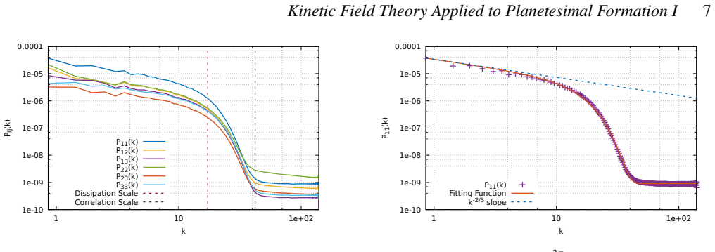
The free generating functional of kinetic field theory, with initial correlations extracted from a streaming-instability snapshot, produces a non-linear density power spectrum $P(k_1,t)$ whose small-scale asymptote is $P(k_1)\sim P_{(0)}(t)/k_1^3$. The slope comes from a saddle-point expansion of the power-spectrum integral: the exponential of the squared free-streaming displacement times the initial momentum covariance matrix satisfies the conditions of an isolated minimum at zero separation with positive-definite Hessian, forcing the $k^{-3}$ form in three dimensions. The amplitude $P_{(0)}(t)$ has an analytic expression and peaks at a finite time, so small-scale structures first grow and then dissolve as particle streams cross. The paper presents this as proof that free streaming from any sufficiently smooth, positive-definite initial momentum covariance inevitably produces scale-invariant clustering below a time-dependent length scale, independent of the specific simulation noise.
Load-bearing premise
The load-bearing premise is that the dust particles truly free-stream, with no gas drag, self-gravity, or particle feedback; if any of those forces act, the universal $k^{-3}$ tail has not been shown to survive.
Editorial extensions
If this is right
- Streaming-instability simulations need not treat the initial particle noise as a source of preferred small-scale structure: below the time-dependent scale $k_0^{-1}$, clustering is scale-invariant by free streaming alone.
- The analytic amplitude formula gives a testable prediction for when small-scale structures reach maximum amplitude, at $t_{\max}\approx 0.97\pi$ in disk units, and when they dissolve.
- The linear power spectrum behaves as $k^{4/3}$ at large scales and $k^{-1}$ at small scales, so the non-linear $k^{-3}$ tail is a genuine non-linear effect of correlated streaming, not an artifact of the linear approximation.
- The method transfers the kinetic field theory formalism from cosmic structure formation to protoplanetary disks, providing a resolution-independent route to clustering statistics in this setting.
Reading between the lines
- If gas drag preserves the $k^{-3}$ tail, the required spatial resolution for streaming-instability simulations would be set by the characteristic scale $k_0^{-1}(t)$ rather than by the initial noise scale, and resolving below it may not change the clustering statistics.
- The same saddle-point argument in two dimensions would predict a $k^{-2}$ tail, giving a dimensional scaling test that could be checked in two-dimensional streaming-instability simulations.
- Scale-invariant clustering of dust below a characteristic length could feed into a scale-free planetesimal mass distribution at the onset of gravitational collapse, connecting the power-spectrum slope to the initial mass function of planetesimals.
- The Gaussianization of the density field (the density variable is the square of a Gaussian variate) suggests the initial density PDF is close to a chi-square-type distribution with one degree of freedom; direct measurements of the density PDF in streaming-instability snapshots could validate or refine the assumed form.
Editorial analysis
A structured set of objections, weighed in public.
Referee Report
Summary. The paper applies Kinetic Field Theory (KFT) to a three-dimensional streaming-instability simulation snapshot, modeling the initial phase-space distribution of dust particles by Gaussianizing the density and momentum fields and fitting isotropic power spectra from the simulation. Restricting the dynamics to freely streaming particles, the authors derive a non-linear density power spectrum and show, via a saddle-point/asymptotic analysis, that it develops a universal k^-3 tail at small scales. They further derive the time-dependent amplitude and onset scale of this tail, and argue that the initial condition of streaming-instability simulations therefore does not imprint a preferred small-scale structure-formation scale.
Significance. If the k^-3 universality claim is correct, the paper offers a valuable analytic handle on small-scale clustering in planetesimal formation: the slope is parameter-free, the amplitude and onset scale are explicit functions of time and of the fitted momentum correlations, and the analytic amplitude is checked against direct numerical integration of the derived expression. The construction of the initial probability distribution from simulation data, including the Gaussianization step and the treatment of density-momentum correlations, is transparent and reusable. The main caveat, acknowledged by the authors, is that the calculation is for free streaming only; the relevance to planetesimal formation depends on whether drag and self-gravity preserve the tail. Because the central claim rests on an asymptotic theorem applied to an approximate spectrum, the technical gaps below must be addressed before the universality statement can be accepted.
major comments (3)
- [Sec. 4.2.1, Eqs. (47)-(49) and (63)] The replacement of the correlation operator C(-i∂_p) by the constant (49) is not justified uniformly in k. The hierarchy in (48) bounds the original Fourier conjugate variable t_pk, but after applying two density operators the relevant argument is L_p = -Σ_j k_j g_qp(t_j) e_j. For an equal-time power spectrum with t1=t2=t and k1+k2=0, one has |L_p| ~ sqrt(2) |k1| t, which is unbounded as k1→∞, precisely the limit used in Sec. 4.2.4 to derive the k^-3 tail. Thus the neglected density-momentum and density-density correlation terms in (B15) may contribute at leading order in the small-scale regime, and the k^-3 result is established only for the approximate Pfree, not for the full KFT expression. The Sec. 5 claim that the SI initial state does not impose a preferred scale is also weakened because scale-dependent density correlations have been removed by this approximation.
- [Sec. 4.2.4, Eqs. (70), (73), (56)-(57)] The asymptotic theorem of Konrad & Bartelmann (2022), as stated in Eq. (70), requires f(x) to be quadratically integrable on R^3 (condition ii). This condition is not satisfied by the function f(r) defined in Eq. (73): since m1(0) and m2(0) are negative while m1(r) and m2(r) tend to zero as r→∞, f(r) tends to the positive constant g_qp^2(t)[-m1(0) - μ^2 m2(0)]. The approximants (56)-(57) have the same property, because a1(r) and a2(r) decay to zero rather than making the difference vanish at infinity. A positive constant is not quadratically integrable on R^3, so the saddle-point expansion (76) is not justified by the cited theorem as written. The authors either need a modified theorem with weaker growth conditions at infinity or an explicit treatment of the boundary contribution from the constant asymptotic value of f.
- [Appendix D, Eqs. (D1)-(D7) and Fig. D1] The assertion that Pdiff can be safely neglected is not established. The integral defining Pdiff is not absolutely convergent: for μ=0 the radial integrand behaves like r^2 e^{y(0)} for large r, and for general μ the oscillatory factor does not produce absolute convergence. The bound in (D3)-(D4) takes the limits k1→∞ and R→∞ simultaneously without a uniform estimate, so it does not prove exponential suppression; moreover, the k1→0 limit computed in (D5)-(D7) diverges, showing that Pdiff is not a harmless finite renormalization. Figure D1 only demonstrates numerical agreement at moderate k (near k≈45) for a single time, whereas the claim concerns k→∞. A rigorous subdominance argument, or a cutoff-independent regularized definition of the full P0, is needed before the full expression (54) can be said to have the k^-3 tail.
minor comments (4)
- [Sec. 3.3.2 and Table 3] The text mentions both c100 and c200 for the density power spectrum fit, but Table 3 lists only c200; please clarify the notation or correct the typo.
- [Eq. (28) and Sec. 3.3.4] The expression for ζ00(r) uses the symbol c200, but the surrounding text and Eq. (26) use c200 with a different subscript convention; please make the notation consistent so the reader can verify the Fourier transform.
- [Figs. 3-5] The k-axis scaling by 2π/L is stated in the main text but not in the figure axis labels; please include the units explicitly on each panel for clarity.
- [Fig. 7 and Sec. 4.2.3] The caption and text refer to the onset of the k^-3 slope near k≈25, but the plotted spectra use a logarithmic axis with different time labels; please add a short description of how k0 in Fig. 8 is extracted from the spectra.
Circularity Check
No significant circularity: the universal k^-3 tail follows from a general asymptotic theorem applied to the assumed Gaussian initial state, not from fitting the target slope.
full rationale
The derivation chain is self-contained in the sense required by the circularity test. The initial iPDF is constructed by Gaussianizing simulation data (Sec. 3.2), and the free-streaming Green's function is specified in Sec. 4.1. The central result, Eq. (63) and its asymptotic tail, is obtained by evaluating the resulting Gaussian integrals and applying a saddle-point/asymptotic theorem from Konrad & Bartelmann (2022). The theorem is a parameter-free mathematical statement whose stated conditions (positive-definite Hessian at an isolated minimum) are checked for the fitted momentum covariance in Eqs. (73)-(75); it does not assume the k^-3 result. Thus the k^-3 slope is a genuine consequence of the smooth, positive covariance input rather than a renamed fit of the same slope. The cited KFT formalism (Bartelmann et al. 2016-2019) is externally established and used as a framework, not as a black-box uniqueness argument. The paper explicitly acknowledges the free-streaming idealization and states that the result may change with interactions (Sec. 5), which is a scope limitation rather than circularity. The main caveats are mathematical: the truncation of the correlation operator uses a bound on t_p that is not uniform in k, and condition (ii) of the cited theorem is not obviously met because f(r) tends to a positive constant. These are correctness risks, not circular reductions of the prediction to its inputs. Accordingly, no specific circular step can be exhibited; the small residual self-citation does not carry the argument by itself.
Assumptions & free parameters
free parameters (5)
- a1, Gaussianization scale for density =
0.1823 ± 0.0005
- a2, Gaussianization offset =
2.569 ± 0.006
- b0, diagonal momentum covariance amplitude =
≈ 1.8 × 10^-5 (disk units)
- b1, off-diagonal momentum covariance amplitude =
≈ 9.2 × 10^-6 (disk units)
- sigma_bar, averaged momentum correlation width =
≈ 10.3 (in units 2π/L)
assumptions (8)
- standard math The KFT generating functional formalism of Martin-Siggia-Rose and the prior KFT results used for density operators and free generating functionals are valid.
- standard math The saddle-point asymptotic theorem of Konrad and Bartelmann (2022) is valid for the integrals considered here.
- domain assumption The SI simulation snapshot can be represented as a statistically homogeneous, isotropic Gaussian random field in phase space after Gaussianizing the density.
- domain assumption Dust particle motion is freely streaming during the times considered; gas drag, self-gravity and particle feedback are neglected.
- domain assumption The specific snapshot (St = 0.01, epsilon0 = 1, eta = 0.05, L = 0.1H, t_snap = 4.25) is representative of general streaming-instability initial states.
- ad hoc to paper The approximation C(p) ≈ constant in Eq. (49) is valid, so density-density correlations at nonzero separation and density-momentum correlations are negligible.
- ad hoc to paper The analytic forms of the power spectra in Eqs. (25)-(27) with fixed exponents alpha = 2/3, beta = 4/3, and alpha_0i = 1/3 represent the simulation statistics.
- ad hoc to paper The Gaussianizing transformation rho = rho_bar^2 with fitted a1 and a2 maps the density distribution to a Gaussian variable.
Cite this review
Pith. "Pith review of Kinetic Field Theory Applied to Planetesimal Formation I: Freely Streaming Dust Particles." pith.science (2026). https://pith.science/paper/HTZ2YGAQ
@misc{pith2026241117514,
  author       = {Pith},
  title        = {Pith review of: Kinetic Field Theory Applied to Planetesimal Formation I: Freely Streaming Dust Particles},
  year         = {2026},
  howpublished = {\url{https://pith.science/paper/HTZ2YGAQ}},
  note         = {Machine review of arXiv:2411.17514}
}
abstract
Planet formation in the solar system was started when the first planetesimals were formed from the gravitational collapse of pebble clouds. Numerical simulations of this process, especially in the framework of streaming instability, produce various power laws for the initial mass function for planetesimals. While recent advances have shed light on turbulence and its role in particle clustering, a comprehensive theoretical framework linking turbulence characteristics to particle cluster properties and planetesimal mass function remains incomplete. Recently, a kinetic field theory for ensembles of point-like classical particles in or out of equilibrium has been applied to cosmic structure formation. This theory encodes the dynamics of a classical particle ensemble by a generating functional specified by the initial probability distribution of particles in phase space and their equations of motion. Here, we apply kinetic field theory to planetesimal formation. A model for the initial probability distribution of dust particles in phase space is obtained from a quasi-initial state for a three-dimensional streaming-instability simulation that is a particle distribution with velocities for gas and particles from the Nakagawa relations. The equations of motion are chosen for the simplest case of freely streaming particles. We calculate the non-linearly evolved density power spectrum of dust particles and find that it develops a universal $k^{-3}$ tail at small scales, suggesting scale-invariant structure formation below a characteristic and time-dependent length scale. Thus, the KFT analysis indicates that the initial state for streaming instability simulations does not impose a constraint on structure evolution during planetesimal formation.
Figures


Figures from the paper (5 more)


Reference graph
Works this paper leans on
-
[1]
, " * write output.state after.block = add.period write newline
ENTRY address author booktitle chapter edition editor howpublished institution journal key month note number organization pages publisher school series title type volume year label extra.label sort.label short.list INTEGERS output.state before.all mid.sentence after.sentence after.block FUNCTION init.state.consts #0 'before.all := #1 'mid.sentence := #2 '...
-
[2]
write newline
" write newline "" before.all 'output.state := FUNCTION n.dashify 't := "" t empty not t #1 #1 substring "-" = t #1 #2 substring "--" = not "--" * t #2 global.max substring 't := t #1 #1 substring "-" = "-" * t #2 global.max substring 't := while if t #1 #1 substring * t #2 global.max substring 't := if while FUNCTION word.in bbl.in " " * FUNCTION format....
-
[3]
M., et al., 2018, @doi [The Astrophysical Journal] 10.3847/2041-8213/aaf741 , 869, L41
Andrews S. M., et al., 2018, @doi [The Astrophysical Journal] 10.3847/2041-8213/aaf741 , 869, L41
-
[4]
Bartelmann M., Fabis F., Berg D., Kozlikin E., Lilow R., Viermann C., 2016, @doi [New Journal of Physics] 10.1088/1367-2630/18/4/043020 , 18, 043020
-
[5]
Bartelmann M., Fabis F., Kozlikin E., Lilow R., Dombrowski J., Mildenberger J., 2017, @doi [New Journal of Physics] 10.1088/1367-2630/aa7e6f , 19, 083001
- [6]
-
[7]
Blum J., Wurm G., 2008, @doi [Annual Review of Astronomy and Astrophysics] https://doi.org/10.1146/annurev.astro.46.060407.145152 , 46, 21
arXiv 2008
-
[8]
Booth R. A., Meru F., Lee M. H., Clarke C. J., 2017, @doi [Monthly Notices of the Royal Astronomical Society] 10.1093/mnras/stx3084 , 475, 167
Show all 41 references
-
[9]
Brandenburg A., Dobler W., 2002, @doi [Computer Physics Communications] https://doi.org/10.1016/S0010-4655(02)00334-X , 147, 471
2002 doi
-
[10]
Dullemond, C
Brauer, F. Dullemond, C. P. Henning, Th. 2008, @doi [A&A] 10.1051/0004-6361:20077759 , 480, 859
2008 doi
-
[11]
N., Hogan R
Cuzzi J. N., Hogan R. C., Shariff K., 2008, @doi [The Astrophysical Journal] 10.1086/591239 , 687, 1432
2008 doi
-
[12]
N., Hogan R
Cuzzi J. N., Hogan R. C., Bottke W. F., 2010, @doi [Icarus] https://doi.org/10.1016/j.icarus.2010.03.005 , 208, 518
2010 doi
-
[13]
P., Mazenko G
Das S. P., Mazenko G. F., 2012, @doi [Journal of Statistical Physics] 10.1007/s10955-012-0610-y , 149, 643
2012 doi
-
[14]
Güttler, C. Blum, J. Zsom, A. Ormel, C. W. Dullemond, C. P. 2010, @doi [A&A] 10.1051/0004-6361/200912852 , 513, A56
2010 doi
-
[15]
N., 2020, @doi [The Astrophysical Journal] 10.3847/1538-4357/ab76c3 , 892, 120
Hartlep T., Cuzzi J. N., 2020, @doi [The Astrophysical Journal] 10.3847/1538-4357/ab76c3 , 892, 120
2020 doi
-
[16]
N., Weston B., 2017, @doi [Phys
Hartlep T., Cuzzi J. N., Weston B., 2017, @doi [Phys. Rev. E] 10.1103/PhysRevE.95.033115 , 95, 033115
2017 doi
-
[17]
C., Cuzzi J
Hogan R. C., Cuzzi J. N., 2007, @doi [Phys. Rev. E] 10.1103/PhysRevE.75.056305 , 75, 056305
2007 doi
-
[18]
C., Cuzzi J
Hogan R. C., Cuzzi J. N., Dobrovolskis A. R., 1999, @doi [Phys. Rev. E] 10.1103/PhysRevE.60.1674 , 60, 1674
1999 doi
-
[19]
F., 2015, @doi [Monthly Notices of the Royal Astronomical Society] 10.1093/mnras/stv2226 , 455, 89
Hopkins P. F., 2015, @doi [Monthly Notices of the Royal Astronomical Society] 10.1093/mnras/stv2226 , 455, 89
2015 doi
-
[20]
Hubbard A., 2013, @doi [Monthly Notices of the Royal Astronomical Society] 10.1093/mnras/stt543 , 432, 1274
2013 doi
-
[21]
Johansen A., Youdin A., 2007, @doi [The Astrophysical Journal] 10.1086/516730 , 662, 627
2007 doi
-
[22]
S., Mac Low M.-M., Klahr H., Henning T., Youdin A., 2007, @doi [ ] 10.1038/nature06086 , https://ui.adsabs.harvard.edu/abs/2007Natur.448.1022J 448, 1022
Johansen A., Oishi J. S., Mac Low M.-M., Klahr H., Henning T., Youdin A., 2007, @doi [ ] 10.1038/nature06086 , https://ui.adsabs.harvard.edu/abs/2007Natur.448.1022J 448, 1022
2007 doi
-
[23]
Klahr H., Schreiber A., 2021, @doi [The Astrophysical Journal] 10.3847/1538-4357/abca9b , 911, 9
2021 doi
-
[24]
Konrad S., Bartelmann M., 2022, @doi [Monthly Notices of the Royal Astronomical Society] 10.1093/mnras/stac1795 , 515, 2578
2022 doi
-
[25]
E., 2019, @doi [The Astrophysical Journal Letters] 10.3847/2041-8213/ab2596 , 878, L30
Krapp L., Benítez-Llambay P., Gressel O., Pessah M. E., 2019, @doi [The Astrophysical Journal Letters] 10.3847/2041-8213/ab2596 , 878, L30
2019 doi
-
[26]
A., Lin D
Kretke K. A., Lin D. N. C., 2007, @doi [The Astrophysical Journal] 10.1086/520718 , 664, L55
2007 doi
-
[27]
C., Siggia E
Martin P. C., Siggia E. D., Rose H. A., 1973, @doi [Phys. Rev. A] 10.1103/PhysRevA.8.423 , 8, 423
1973 doi
-
[28]
P., Lovascio F., Paardekooper S.-J., 2021, @doi [Monthly Notices of the Royal Astronomical Society] 10.1093/mnras/stab112 , 502, 1469
McNally C. P., Lovascio F., Paardekooper S.-J., 2021, @doi [Monthly Notices of the Royal Astronomical Society] 10.1093/mnras/stab112 , 502, 1469
2021 doi
-
[29]
F., Nesvorný D., Levison H
Morbidelli A., Bottke W. F., Nesvorný D., Levison H. F., 2009, @doi [Icarus] https://doi.org/10.1016/j.icarus.2009.07.011 , 204, 558
2009 doi
-
[30]
Nakagawa Y., Sekiya M., Hayashi C., 1986, @doi [Icarus] https://doi.org/10.1016/0019-1035(86)90121-1 , 67, 375
1986 doi
-
[31]
P., Lovascio F., 2020, @doi [Monthly Notices of the Royal Astronomical Society] 10.1093/mnras/staa3162 , 499, 4223
Paardekooper S.-J., McNally C. P., Lovascio F., 2020, @doi [Monthly Notices of the Royal Astronomical Society] 10.1093/mnras/staa3162 , 499, 4223
2020 doi
-
[32]
G., Norman M
Pan L., Padoan P., Scalo J., Kritsuk A. G., Norman M. L., 2011, @doi [The Astrophysical Journal] 10.1088/0004-637x/740/1/6 , 740, 6
2011 doi
-
[33]
Partnership A., et al., 2015, @doi [The Astrophysical Journal Letters] 10.1088/2041-8205/808/1/L3 , 808, L3
2015 doi
-
[34]
Schreiber A., 2018, PhD thesis, MPI for Astronomy, @doi 10.11588/heidok.00024579 , urn:nbn:de:bsz:16-heidok-245792
2018 doi
-
[35]
R., 1997, @doi [Journal of Fluid Mechanics] 10.1017/S0022112096004454 , https://ui.adsabs.harvard.edu/abs/1997JFM...335...75S 335, 75
Sundaram S., Collins L. R., 1997, @doi [Journal of Fluid Mechanics] 10.1017/S0022112096004454 , https://ui.adsabs.harvard.edu/abs/1997JFM...335...75S 335, 75
1997 doi
-
[36]
J., 1977, @doi [Monthly Notices of the Royal Astronomical Society] 10.1093/mnras/180.2.57 , 180, 57
Weidenschilling S. J., 1977, @doi [Monthly Notices of the Royal Astronomical Society] 10.1093/mnras/180.2.57 , 180, 57
1977 doi
-
[37]
L., 1972, in Elvius A., ed., From Plasma to Planet
Whipple F. L., 1972, in Elvius A., ed., From Plasma to Planet. p. 211
1972
-
[38]
Johansen, A
Yang, C.-C. Johansen, A. Carrera, D. 2017, @doi [A&A] 10.1051/0004-6361/201630106 , 606, A80
2017 doi
-
[39]
N., Goodman J., 2005, @doi [The Astrophysical Journal] 10.1086/426895 , 620, 459
Youdin A. N., Goodman J., 2005, @doi [The Astrophysical Journal] 10.1086/426895 , 620, 459
2005 doi
-
[40]
Youdin A., Johansen A., 2007, @doi [The Astrophysical Journal] 10.1086/516729 , 662, 613
2007 doi
-
[41]
Zhu Z., Yang C.-C., 2020, @doi [Monthly Notices of the Royal Astronomical Society] 10.1093/mnras/staa3628 , 501, 467
2020 doi
Reviewed August 12, 2026 · model on record in the stance chip above.
Discussion (0). Continue with ORCID to comment.