REVIEW 4 major objections 5 minor 44 references
A geometric approach to estimate background in astronomical images
T0 review · 4 major / 5 minor · reviewed 2026-08-12 · deepseek-v4-flash
Pith's one-line read A geometric minima estimator recovers astronomical background within 10-14% where 3-sigma clipping fails.
desk verdict Solid minima-sampling background estimator, but the headline 10-14% accuracy is calibrated to one smoothing configuration and needs a mapping for F before it generalizes. read the letter →
The pith
A machine-rendered reading of the paper's core claim, the machinery that carries it, and where it could break.
The reading
What carries the argument
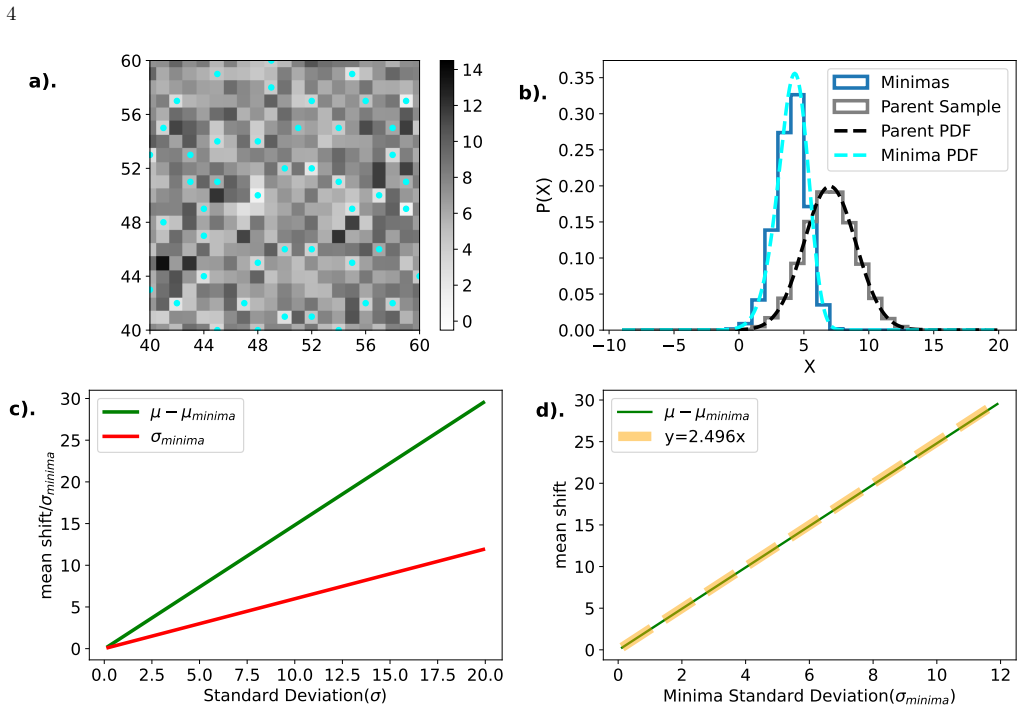
The load-bearing object is the minima distribution of a random field and the identity $P_{\rm min}(x) = N P(x)(1-\Phi(x))^n$, which gives the isomorphic CDF relation $\Phi = 1 - (1 - \Phi_{\rm min})^{1/(n+1)}$ and the linear moment-shift law $\mu = \mu_{\rm min} + K\sigma_{\rm min}$. The operative mechanism in real images is the iterative smoothed-minima search: wide-to-narrow Gaussian smoothing with steepest descent, followed by fixed box sampling at the final minima, which targets source-free regions without collapsing the 2D pixel distribution into a 1D histogram. The quantitative claim is carried by empirically fitted coefficients: $K \approx 2.496$, the Poisson correction $A \approx 0.231$ and $\gamma \approx -0.2085$, and, for the smoothed-field recipe, the mean-shift coefficient $F = 0.213$ with the $\sigma$ offset $\sqrt{\lambda} = \sigma_{\rm min} + 0.1$.
What would settle it
Generate a Poisson background image with known $\lambda$ from 0.03 to 100, with sources injected as in the paper, but run the recipe with a different final kernel and box size (for example $G_2$ FWHM = 6 pixels and $b = 15$ pixels); if the recovered background leaves the paper's 10-14% band, the claimed accuracy is not a general property of the method.
Extended reading notes
Core claim
The central discovery is a statistical relation between a random field and its local minima: for an $M$-dimensional iid field, the minima PDF is $P_{\rm min}(x) = N P(x)(1-\Phi(x))^n$, and the minima CDF is isomorphic to the parent CDF, so the parent mean can be recovered as $\mu = \mu_{\rm min} + K\sigma_{\rm min}$, with $K \approx 2.496$ for Gaussian fields and a Poisson correction $\lambda \approx \mu_{\rm min} + 2.496\sigma_{\rm min} + A\mu_{\rm min}^{\gamma}$ ($A \approx 0.231$, $\gamma \approx -0.2085$). For images with sources, the paper replaces direct minima sampling with an iterative recipe: smooth with a wide Gaussian kernel (full width at half maximum 15.3 pixels), find minima by steepest descent, then re-find minima through progressively narrower kernels down to 3.5 pixels, and sample $7 \times 7$ pixel boxes around the final minima. On simulated UVIT-like images this recovers the input background within about 10% at $\lambda = 0.348$ in an uncrowded field, within 14% at $\lambda = 0.348$ in a crowded field, within about 10% at $\lambda = 5.8$ in a crowded field, and within 0.65% at $\lambda = 5.8$ uncrowded.
Load-bearing premise
The 10-14% accuracy claims rest on empirically fitted constants ($A \approx 0.231$, $\gamma \approx -0.2085$, the 0.1 $\sigma$ offset, and especially $F = 0.213$) that are calibrated to one fixed smoothing sequence and box size, with no closed-form mapping for other settings.
Editorial extensions
If this is right
- Low-photon UV images with $\lambda \approx 0.35$ and sparse sources get a background estimate within about 10%, whereas histogram-clipping routines return values orders of magnitude too low.
- Crowded fields near 500 sources per square arcminute get recovered background within about 14% at low $\lambda$ and about 10% at higher $\lambda$, instead of the roughly 200% and 60% overestimates of clipping-based estimators.
- Source contamination in the sampled pixels stays one to two orders of magnitude below that of 3-sigma clipping, improving the signal-to-noise of faint sources near the detection limit.
- The method extends to spatially varying backgrounds by patching the field and interpolating, producing background and rms maps for a 236 square arcminute field in about 30 seconds.
- The paper proposes the minima routine for wide deep surveys where faint-source density is high, naming Euclid, DESI imaging, and LSST as suitable applications.
Reading between the lines
- Because the minima CDF is isomorphic to the parent CDF for any continuous parent distribution, the same moment-correction logic should apply to non-Poisson noise mixtures such as read noise and dark current, provided the coefficients are recalibrated; the paper calibrates only Gaussian and Poisson cases.
- The fitted coefficients $F$, $A$, and $\gamma$ are measurements rather than derivations, so a closed-form mapping from kernel widths and box size to $F$ would let the method be used without per-instrument recalibration; the paper's Appendix leaves that mapping open.
- The residual deviation near $\lambda \approx 0.1$ is likely set by integer-count zeros; an exposure-time-aware version of the offset in $\sqrt{\lambda} = \sigma_{\rm min} + 0.1$ would be a direct testable extension for very short exposures.
- The paper's reported accuracy concerns recovering the mean background; survey decisions depend at least as much on patch-to-patch variance and on correlated noise from artifacts, which the paper lists as an untested limitation.
Editorial analysis
A structured set of objections, weighed in public.
Referee Report
Summary. The manuscript presents a geometric method for estimating astronomical background levels by identifying local minima via steepest descent and exploiting the statistics of these minima to recover the parent distribution's mean. For IID Gaussian fields the authors derive an analytic recovery relation μ = μ_min + 2.496 σ_min (Eq. 16) and verify it numerically. For Poisson noise they add an empirical power-law correction (Eq. 18). For crowded and low-count fields they propose a multi-resolution recipe: locate minima on a heavily smoothed image, track them through progressively narrower kernels, and sample boxes around the final minima on the original image; the sampled mean is corrected by an empirical relation (Eq. 24). The method is tested on simulated Poisson fields and UVIT-like images with injected Sérsic sources, reporting recovery within 10% (uncrowded, λ=0.348) and 14% (crowded) of the input background, while SExtractor's background shows much larger deviations. A background-map extension and several limitations are discussed.
Significance. The central idea of using 2D spatially selected minima to avoid source contamination is a genuine methodological contribution, and the analytic Gaussian result (K≈2.496) provides a clean, numerically checked asymptotic baseline. The contamination-fraction comparison (Fig. 8) convincingly demonstrates that the minima sampler collects 1–2 orders of magnitude less source flux than SExtractor's 3σ-clipping over the tested range, which is the paper's most promising result. The paper honestly lists important limitations (λ≲0.1 failure, crowded-field degradation, diffuse-object caveats). However, the headline 10% and 14% accuracies are currently calibrated for a single smoothing/box configuration and a specific simulated source model, and a sign error in Eq. (15) affects the printed Gaussian derivation. With these issues addressed, the method could be a useful tool for low-count UV surveys.
major comments (4)
- [Section 2.2, Eq. (15)] The printed formula for σ_min contains a sign error. For the minimum of N=9 IID Gaussians, the variance is σ_min^2 = 18 σ^2 ∫_0^1 [Erf^{-1}(2Φ−1)]^2 (1−Φ)^8 dΦ − (μ−μ_min)^2, whereas Eq. (15) as written puts a minus sign before the 18, making the right-hand side negative for a non-negative integrand and producing an imaginary σ_min. This is load-bearing for the central recovery constant K=C/D: the reported numerical values C_gaussian=1.48501 and D_gaussian=0.59779 cannot follow from the printed formula. Please correct the sign and confirm the derivation.
- [Appendix A and Eq. (22)] The quantitative recovery relations used for the source-free and crowded-field tests are μ−μ_min = (0.213±0.002)σ (Eq. 22) and λ_recovery = μ_min + 0.213(σ_min + 0.1) (Eq. 24), with the constant 0.213 fitted for one configuration: G1 FWHM=15.3 px, G2 FWHM=3.5 px, b=7 px. Appendix A shows only qualitative dependencies of F on G1, G2, and b (Figs. 11–12) and gives no closed-form mapping or tabulated values. Consequently the abstract's 'within 10%' and 'within 14%' claims are properties of this single calibration, not of the geometric minima method as presented. A user applying the stated '5–10× PSF' prescription at a different pixel scale or PSF cannot compute F and has no accuracy guarantee. Please provide at least a fitted formula or lookup table for F(G1,G2,b) over the tested ranges, or explicitly restrict the claimed accuracy to the tested configuration.
- [Section 4.3, Eq. (25)] The background recovery equation includes a source contamination term Sc, but the paper states that Sc 'cannot be estimated independently of the background.' The implementation therefore does not correct for Sc; it only attempts to minimize it by sampling near minima. The claimed 10–14% accuracies in Table 1 are for a specific simulated source model (Gaussian PSF, SNR 0.7–7, one source-count value for each crowding level) with no independent estimate of Sc. Since the Discussion acknowledges that the source distribution and PSF 'could have a significant impact' on background estimation, the paper should either provide a method to estimate or bound Sc, or revise the claims to state they are validation results for the simulation setup, not universal accuracy guarantees.
- [Section 4.4 and Table 1] The text states the Minima routine recovers B_MS = 1.03×10^-4 cps/pixel for the 500-source, texp=3000 s image (figure 10a), while Table 1 lists 1.05×10^-4; the corresponding deviations are ~11% and 9.32% from the input 1.16×10^-4, so the abstract's 'within 10%' claim is sensitive to this discrepancy. Additionally, each entry in Table 1 appears to be a single realization (or a single averaged value) with no repeated-trial statistics, uncertainties, or scatter; the reader cannot assess whether the 10–14% figures are robust. Please reconcile the printed values and report mean ± scatter over multiple realizations.
minor comments (5)
- [Section 2.2, Eq. (14)] The integral contains a stray '(Φ)' after Erf^{-1}(2Φ−1); it should read ∫_0^1 Erf^{-1}(2Φ−1) (1−Φ)^8 dΦ.
- [Section 4.3, after Figure 7] The text 'images containing 500, 2000 and 4000 thousand sources' should read '4000 sources'; similarly, the phrase in Section 3 '300 to 3600 (69 to 828 sources/arcminutes²)' should clarify the units of source density.
- [Section 4.2, Eq. (23)] The offset 0.1 is not dimensionless; the paper notes it becomes 0.1/texp for cps units, but the units should be stated explicitly in the equation itself.
- [Abstract and Section 5] The claims of 'within 10%' for low-photon-count images should be accompanied by the λ≳0.1 applicability restriction stated in Section 5, since the paper itself says the method is not confident below λ~0.1.
- [References] The bibliography lists Saha et al. 2024a and 2024b with the same arXiv identifier (arXiv:2408.03629); please verify the citations.
Circularity Check
No significant circularity: the analytic minima relations are derived independently, and the headline recovery figures are tested on separately generated source-injected images.
full rationale
The central derivation chain is self-contained. Section 2 derives the minima distribution from the parent probability distribution via Equation (1), obtains the isomorphic CDF relation in Equation (3), and computes the Gaussian mean-shift coefficient K = 2.496 analytically from Equations (14)-(16). The Poisson corrections (A ≈ 0.231, γ ≈ -0.2085 in Equation 18) and the Section 4 empirical coefficients (F = 0.213 in Equation 22 and the 0.1 offset in Equation 23) are fitted to simulated Poisson fields, but the paper explicitly labels them as empirical relations rather than first-principles derivations. The headline claims of 10% and 14% recovery come from separately generated source-injected and UVIT-like images with known input backgrounds, not from the same fields used for the fitting, so those tests are external benchmarks rather than forced restatements of the calibration. The unestimated source-contamination term Sc in Equation (25) is a stated limitation and generalizability concern, but it does not make the recovery circular. Load-bearing citations are to standard algorithms and data sources, not to a self-referential uniqueness or existence claim. Therefore the paper's derivation and validation do not reduce to their own inputs by construction.
Assumptions & free parameters
free parameters (5)
- A, gamma (Poisson power-law correction) =
A ≈ 0.231, γ ≈ -0.2085
- Poisson sigma offset =
0.1
- Mean-shift coefficient F =
0.213 ± 0.002
- Smoothing kernels and box size (G1, G2, b) =
G1 FWHM=15.3 px, G2 FWHM=3.5 px, b=7 px
- Source-masking clipping thresholds =
3-sigma on max flux and segment area
assumptions (4)
- domain assumption Background pixels are IID draws from a single continuous (or Poisson) distribution within a patch.
- standard math The order-statistics formula P_min = (n+1) P(x) (1-Φ(x))^n holds for continuous distributions with independent neighbors.
- domain assumption Local minima of the smoothed image are reliable indicators of source-free regions.
- domain assumption Sources are localized clumps that can be masked via maxima segmentation; very diffuse objects were not considered.
Cite this review
Pith. "Pith review of A geometric approach to estimate background in astronomical images." pith.science (2026). https://pith.science/paper/JZX3DTJU
@misc{pith2026241117566,
  author       = {Pith},
  title        = {Pith review of: A geometric approach to estimate background in astronomical images},
  year         = {2026},
  howpublished = {\url{https://pith.science/paper/JZX3DTJU}},
  note         = {Machine review of arXiv:2411.17566}
}
abstract
Estimating the true background in an astronomical image is fundamental to detecting faint sources. In a typical low-photon count astronomical image, such as in the far and near-ultraviolet wavelength range, conventional methods relying on the 3-sigma clipping and median or mode estimation often fail to capture the true background level accurately. As a consequence, differentiating true sources from noise peaks remains a challenging task. Additionally, in such images, effectively identifying and excluding faint sources during the background estimation process remains crucial, as undetected faint sources could contaminate the background. This results in overestimating the true background and obscuring the detection of very faint sources. To tackle this problem, we introduce a geometric approach based on the method of steepest descent to identify local minima in an astronomical image. The proposed algorithm based on the minima statistics effectively reduces the confusion between sources and background in the image; thereby ensuring a better background estimation and enhancing the reliability of faint source detection. Our algorithm performs well compared to conventional methods in estimating the background even in crowded field images. In low-photon count, less crowded images, our algorithm recovers the background within 10\%, while traditional methods drastically underestimate it by a few orders of magnitude. In crowded fields, the conventional methods overestimates the background by $\sim 200\%$ whereas our algorithm recovers the true background within $\sim 14\%$. We provide a simple prescription to create a background map using our algorithm and discuss its application in large astronomical surveys.
Figures


Figures from the paper (9 more)


Reference graph
Works this paper leans on
-
[1]
2015, ApJS, 220, 1, doi: 10.1088/0067-0049/220/1/1
Akhlaghi, M., & Ichikawa, T. 2015, ApJS, 220, 1, doi: 10.1088/0067-0049/220/1/1
-
[2]
1993, MNRAS, 265, 641, doi: 10.1093/mnras/265.3.641 Astropy Collaboration, Price-Whelan, A
Almoznino, E., Loinger, F., & Brosch, N. 1993, MNRAS, 265, 641, doi: 10.1093/mnras/265.3.641 Astropy Collaboration, Price-Whelan, A. M., Lim, P. L., et al. 2022, ApJ, 935, 167, doi: 10.3847/1538-4357/ac7c74
-
[3]
Berry, D. S. 2015, Astronomy and Computing, 10, 22, doi: 10.1016/j.ascom.2014.11.004
-
[4]
1996, A&AS, 117, 393, doi: 10.1051/aas:1996164
Bertin, E., & Arnouts, S. 1996, A&AS, 117, 393, doi: 10.1051/aas:1996164
-
[5]
2019, A&A, 621, A133, doi: 10.1051/0004-6361/201834312
Borlaff, A., Trujillo, I., Rom´ an, J., et al. 2019, A&A, 621, A133, doi: 10.1051/0004-6361/201834312
-
[6]
Boulanger, F., Cox, P., & Jones, A. P. 2000, in Infrared Space Astronomy, Today and Tomorrow, ed. F. Casoli, J. Lequeux, & F. David, Vol. 70, 251
work page 2000
-
[7]
Bouwens, R. J., Illingworth, G. D., Oesch, P. A., et al. 2012, ApJL, 752, L5, doi: 10.1088/2041-8205/752/1/L5
-
[8]
Dey, A., Schlegel, D. J., Lang, D., et al. 2019, AJ, 157, 168, doi: 10.3847/1538-3881/ab089d
Show all 44 references
-
[9]
2024, arXiv e-prints, arXiv:2401.13269, doi: 10.48550/arXiv.2401.13269 Euclid Collaboration, Borlaff, A
Dhiwar, S., Saha, K., Maulick, S., et al. 2024, arXiv e-prints, arXiv:2401.13269, doi: 10.48550/arXiv.2401.13269 Euclid Collaboration, Borlaff, A. S., G´ omez-Alvarez, P., et al. 2022, A&A, 657, A92, doi: 10.1051/0004-6361/202141935
-
[10]
P., Brown, T
Gardner, J. P., Brown, T. M., & Ferguson, H. C. 2000, ApJL, 542, L79, doi: 10.1086/312930
2000 doi
-
[11]
K., Tandon, S
Ghosh, S. K., Tandon, S. N., Singh, S. K., et al. 2022, Journal of Astrophysics and Astronomy, 43, 77, doi: 10.1007/s12036-022-09842-7
2022 doi
-
[12]
Howell, S. B. 2006, Handbook of CCD Astronomy, Vol. 5
2006
-
[13]
2023, MNRAS, 523, 6310, doi: 10.1093/mnras/stad1692
Ikeda, R., Morishita, T., Tsukui, T., et al. 2023, MNRAS, 523, 6310, doi: 10.1093/mnras/stad1692
2023 doi
-
[14]
1997, ARA&A, 35, 267, doi: 10.1146/annurev.astro.35.1.267 Ivezi´ c,ˇZ., Kahn, S
Impey, C., & Bothun, G. 1997, ARA&A, 35, 267, doi: 10.1146/annurev.astro.35.1.267 Ivezi´ c,ˇZ., Kahn, S. M., Tyson, J. A., et al. 2019, ApJ, 873, 111, doi: 10.3847/1538-4357/ab042c
1997 doi
-
[15]
Jacoby, G. H., ed. 1990, CCDs in astronomy : proceedings of a conference held in Tuscon, Arizona, 6-8 September 1989, Vol. 8
1990
-
[16]
J., & Tyson, J
Ji, I., Hasan, I., Schmidt, S. J., & Tyson, J. A. 2018, PASP, 130, 084504, doi: 10.1088/1538-3873/aac4ed
2018 doi
-
[17]
Jones, R. C. 1958, Journal of the Optical Society of America (1917-1983), 48, 934 17
1958
-
[18]
S., Hasan, I., & Tyson, J
Kelvin, L. S., Hasan, I., & Tyson, J. A. 2023, MNRAS, 520, 2484, doi: 10.1093/mnras/stad180
2023 doi
-
[19]
2015, ApJL, 807, L2, doi: 10.1088/2041-8205/807/1/L2
Koda, J., Yagi, M., Yamanoi, H., & Komiyama, Y. 2015, ApJL, 807, L2, doi: 10.1088/2041-8205/807/1/L2
2015 doi
-
[20]
Kormendy, J., & Bahcall, J. N. 1974, AJ, 79, 671, doi: 10.1086/111595
1974 doi
-
[21]
K., et al
Leinert, C., Bowyer, S., Haikala, L. K., et al. 1998, A&AS, 127, 1, doi: 10.1051/aas:1998105
1998 doi
-
[22]
I., Starck, J.-L., & Kilbinger, M
Liaudat, T. I., Starck, J.-L., & Kilbinger, M. 2023, Frontiers in Astronomy and Space Sciences, 10, 1158213, doi: 10.3389/fspas.2023.1158213
2023
-
[23]
2000, MNRAS, 312, L9, doi: 10.1046/j.1365-8711.2000.03268.x
Madau, P., & Pozzetti, L. 2000, MNRAS, 312, L9, doi: 10.1046/j.1365-8711.2000.03268.x
2000
-
[24]
1959, Proceedings of the Physical Society, 74, 233, doi: 10.1088/0370-1328/74/3/301
Mandel, L. 1959, Proceedings of the Physical Society, 74, 233, doi: 10.1088/0370-1328/74/3/301
1959 doi
-
[25]
E., Spavone, M., et al
Martin, G., Bazkiaei, A. E., Spavone, M., et al. 2022, MNRAS, 513, 1459, doi: 10.1093/mnras/stac1003
2022 doi
-
[26]
2018, AJ, 156, 86, doi: 10.3847/1538-3881/aad0f0
Matsumoto, T., Tsumura, K., Matsuoka, Y., & Pyo, J. 2018, AJ, 156, 86, doi: 10.3847/1538-3881/aad0f0
2018 doi
-
[27]
2023, ApJS, 264, 40, doi: 10.3847/1538-4365/aca7c4
Mondal, C., Saha, K., Bhattacharya, S., et al. 2023, ApJS, 264, 40, doi: 10.3847/1538-4365/aca7c4
2023 doi
-
[28]
2014, ApJS, 213, 32, doi: 10.1088/0067-0049/213/2/32 O’Donoghue, D
Murthy, J. 2014, ApJS, 213, 32, doi: 10.1088/0067-0049/213/2/32 O’Donoghue, D. 1995, Baltic Astronomy, 4, 519, doi: 10.1515/astro-1995-0411
2014 doi
-
[29]
2018, MNRAS, 478, 4657, doi: 10.1093/mnras/sty1139
Pahwa, I., & Saha, K. 2018, MNRAS, 478, 4657, doi: 10.1093/mnras/sty1139
2018 doi
-
[30]
2008, A&A, 481, 575, doi: 10.1051/0004-6361:20079279
Patat, F. 2008, A&A, 481, 575, doi: 10.1051/0004-6361:20079279
2008 doi
-
[31]
1996, PASP, 108, 699, doi: 10.1086/133788
Racine, R. 1996, PASP, 108, 699, doi: 10.1086/133788
1996 doi
-
[32]
I., Gardner, J
Rafelski, M., Teplitz, H. I., Gardner, J. P., et al. 2015, AJ, 150, 31, doi: 10.1088/0004-6256/150/1/31
2015 doi
-
[33]
2021, Journal of Astrophysics and Astronomy, 42, 59, doi: 10.1007/s12036-021-09715-5
Saha, K., Dhiwar, S., Barway, S., Narayan, C., & Tandon, S. 2021, Journal of Astrophysics and Astronomy, 42, 59, doi: 10.1007/s12036-021-09715-5
2021 doi
- [34]
-
[35]
2014, A&A, 567, A97, doi: 10.1051/0004-6361/201423429
Sandin, C. 2014, A&A, 567, A97, doi: 10.1051/0004-6361/201423429
2014 doi
-
[36]
1918, Annalen der Physik, 362, 541, doi: 10.1002/andp.19183622304
Schottky, W. 1918, Annalen der Physik, 362, 541, doi: 10.1002/andp.19183622304
1918 doi
-
[37]
T., Harding, P., & Mihos, J
Slater, C. T., Harding, P., & Mihos, J. C. 2009, PASP, 121, 1267, doi: 10.1086/648457
2009 doi
-
[38]
Stetson, P. B. 1987, PASP, 99, 191, doi: 10.1086/131977
1987 doi
-
[39]
Tyson, J. A. 1984, PASP, 96, 566, doi: 10.1086/131382 V¨ ais¨ anen, P., Tollestrup, E. V., & Fazio, G. G. 2001, MNRAS, 325, 1241, doi: 10.1046/j.1365-8711.2001.04566.x van Dokkum, P. G., Abraham, R., Merritt, A., et al. 2015, ApJL, 798, L45, doi: 10.1088/2041-8205/798/2/L45
1984
-
[40]
E., et al
Virtanen, P., Gommers, R., Oliphant, T. E., et al. 2020, Nature Methods, 17, 261, doi: 10.1038/s41592-019-0686-2
2020 doi
-
[41]
E., Kaviraj, S., Collins, C
Watkins, A. E., Kaviraj, S., Collins, C. C., et al. 2024, MNRAS, 528, 4289, doi: 10.1093/mnras/stae236
2024 doi
-
[42]
K., Donas, J., Arnouts, S., et al
Xu, C. K., Donas, J., Arnouts, S., et al. 2005, ApJL, 619, L11, doi: 10.1086/425252
2005 doi
-
[43]
2014, MNRAS, 443, L20, doi: 10.1093/mnrasl/slu073
Yue, B., Ferrara, A., Vanzella, E., & Salvaterra, R. 2014, MNRAS, 443, L20, doi: 10.1093/mnrasl/slu073
2014 doi
-
[44]
2021, ApJS, 257, 60, doi: 10.3847/1538-4365/ac2607 18 APPENDIX A
Zaritsky, D., Donnerstein, R., Karunakaran, A., et al. 2021, ApJS, 257, 60, doi: 10.3847/1538-4365/ac2607 18 APPENDIX A. THE MEAN SHIFT COEFFICIENT AND SIGMA RATIO FOR GAUSSIAN RANDOM FIELDS To estimate background using the smoothed image minima in section 4, we introduce the ...
2021 doi
Reviewed August 12, 2026 · model on record in the stance chip above.
Discussion (0). Continue with ORCID to comment.