Comparison of Tiny Machine Learning Techniques for Embedded Acoustic Emission Analysis

Luciano Sebastian Martinez-Rau; Sebastian Bader; Uditha Muthumala; Yuxuan Zhang

REVIEW 4 major objections 4 minor 17 references

Comparison of Tiny Machine Learning Techniques for Embedded Acoustic Emission Analysis

T0 review · 4 major / 4 minor · reviewed 2026-08-12 · deepseek-v4-flash

Challenge this review Re-run · record.json Download PDF Read on arXiv ↗ Review JSON

Pith's one-line read The paper claims that for embedded acoustic-emission classification, feeding raw waveforms to a tiny neural network yields 52-71x lower energy per prediction than feature-based inputs, at the cost of a larger memory footprint.

desk verdict Useful empirical comparison, but the headline speed/energy claim likely rests on an unoptimized feature-extraction implementation that makes the comparison unfair. read the letter →

arxiv 2411.17733 v1 pith:LCW2CTFA submitted 2024-11-22 eess.SP cs.LGeess.AS

Uditha Muthumala , Yuxuan Zhang , Luciano Sebastian Martinez-Rau , Sebastian Bader This is my paper · ORCID

classification eess.SPcs.LGeess.AS

keywords TinyMLacousticemissionstructuralhealthmonitoringfeatureextractionembeddedmachinelearningenergyconsumptionedgeinferenceconcretedamageclassification

verification ladder T0 review T1 audit T2 compute T3 formal

The pith

A machine-rendered reading of the paper's core claim, the machinery that carries it, and where it could break.

The reading

This paper asks a practical question for deploying machine learning on battery-powered structural-health sensors: should a microcontroller classify acoustic-emission signals from raw waveforms, or from a small set of engineered features? On a standard Arduino-class board, the authors find that all three compared models classify concrete damage types with over 99% accuracy, but the choice is decided by the whole pipeline, not the neural network alone. The raw-signal model, which skips feature extraction, completes a prediction in about 6.7 ms and consumes about 0.073 mJ, while feature-based models spend 345-473 ms extracting features and consume 3.79-5.19 mJ per prediction. The paper concludes that raw-signal input is the preferred TinyML approach for this application when the larger memory footprint is acceptable.

What carries the argument

The comparison's load-bearing mechanism is the embedded feature-extraction pipeline: custom C implementations of statistical, temporal, and frequency-domain features (with an FFT library for the frequency features) running on the microcontroller before the neural net. Because this pipeline runs in floating point on every captured signal, its execution time dwarfs the int8-quantized inference kernel, making feature extraction the bottleneck that determines total time and energy. The models themselves are feed-forward ANNs with two hidden layers, optimized by hyperparameter search and quantized to 8-bit integers for microcontroller deployment.

What would settle it

Measure the nRF52840's current draw separately during int8 inference and during floating-point C feature extraction, then recompute energy per prediction using the per-phase currents and the durations in Table II; if feature extraction's current substantially exceeds inference current, the raw-signal model's energy advantage shrinks toward or below the time ratio of 52-71x.

Watch

Extended reading notes

Core claim

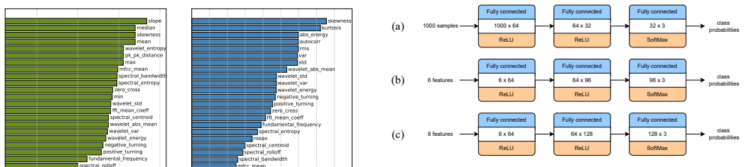
On an Arduino Nano 33 BLE Sense (nRF52840, Cortex-M4), the authors deploy three int8-quantized feed-forward neural networks for classifying acoustic emissions from a concrete block as tensile, shear, or mixed damage. The raw-signal model takes 1000 samples per waveform as input and reaches 99.6% test accuracy with 66,243 parameters; the 6-feature and 8-feature models reach 99.2% and 99.1% accuracy with 6,979 and 9,283 parameters. Pure inference is faster for the feature models (767-930 microseconds vs 6,656 microseconds), but the embedded feature-extraction code dominates: 471,937 microseconds for the six time/frequency features and 344,106 microseconds for the eight time-domain features. Consequently the raw-signal model's total processing time is 6,656 microseconds versus 345,036-472,704 microseconds, and its estimated energy per inference is 0.073 mJ versus 3.79-5.19 mJ, a 52-71x advantage.

Load-bearing premise

The energy comparison assumes the microcontroller draws a constant power from the datasheet, so energy is just processing time scaled by one fixed current; if feature-extraction code draws more or less current than the int8 inference kernel, the reported 52-71x energy advantage changes.

Editorial extensions

If this is right

Raw-signal TinyML models are a practical option for real-time structural health monitoring on common low-power microcontrollers, as long as roughly 223 KB of flash and 126 KB of RAM are available.
Total pipeline time, not model inference time, is the deciding metric for battery-powered IoT; optimizing the model alone can be pointless if feature extraction dominates.
Dropping frequency-domain features and the FFT reduces total processing time by roughly 127 ms and energy by about 27% compared with the 6-feature model, while keeping accuracy essentially unchanged.
The high accuracies of all models (at least 99.1%) show that both raw waveforms and a carefully selected small feature set carry enough information for damage-type classification.

Reading between the lines

Editorial extensions of the paper, not claims the author makes directly.

If the energy estimate were refined by measuring actual current during feature extraction and inference separately, the qualitative ranking would likely stand, but the 52-71x margin is only as accurate as the fixed-power assumption.
The same 'preprocessing dominates' effect should generalize to other edge-sensing applications: any expensive signal-conditioning step on a microcontroller can outweigh a small neural network, so system cost, not model cost, should drive architecture choices.
A direct testable extension would replace the custom floating-point C feature extraction with fixed-point or hardware-accelerated FFT; if feature extraction then dropped below raw inference time, the preferred-input conclusion could reverse on other hardware.

Share X Bluesky LinkedIn Reddit HN

Editorial analysis

A structured set of objections, weighed in public.

Desk editor's note, referee report, and a circularity audit.

Desk Editor's Note

read the letter

The useful nugget in this paper is the first apples-to-apples comparison of raw-waveform and hand-crafted-feature ANNs for acoustic emission classification on a Cortex-M4, with accuracies, model sizes, and timings. The dataset is public, the confusion matrices look consistent, and the result that eight time-domain features match a set containing an FFT feature is a nice, reproducible observation.

But the central speed/energy claim has a fairness problem. The raw-input model runs on int8 TFLM, a heavily optimized inference engine. The feature models run on hand-written C that the paper calls 'optimized' but gives no clock frequency, compiler flags, or microbenchmark. Eight O(n) time-domain features over 1000 samples taking 344 ms is roughly two orders of magnitude slower than a straightforward float implementation on the same 64 MHz M4F. That points to double-precision math and pow(x,4) for kurtosis rather than any inherent cost of feature extraction. If the features were implemented with single-pass integer arithmetic or CMSIS-DSP, the 52-71x speed and energy gap would shrink dramatically, and the paper's main conclusion would wobble.

The reader flagged the constant-power energy assumption, which is real but secondary: energy is time times a datasheet current, so it inherits the timing problem. More minor issues: the 6-feature set lists only five features, leaving the model input ambiguous; and RFE appears to run on the full dataset before the train/test split, which could leak test information into feature selection. Both are fixable.

Credit where due: the classification results themselves (all over 99%) are plausible, the models are small enough for the target node, and the comparison of memory footprints is useful. The paper is honest in that it reports its methods, but the missing benchmark details are exactly what matters for an empirical claim like this.

Bottom line: this deserves peer review, but only if the authors are pushed to redo the feature-extraction timing with a properly optimized implementation and to report measurement conditions. I would not cite the energy conclusion until that is done. Worth a reading-group discussion, though, because the failure mode is instructive.

Referee Report

4 major / 4 minor

Summary. The manuscript compares three approaches for classifying acoustic emission (AE) signals on a low-power embedded platform (Arduino Nano 33 BLE Sense / nRF52840): (i) a fully-connected ANN operating on 1000 raw signal samples, (ii) an ANN on six selected time/frequency-domain features, and (iii) an ANN on eight time-domain features. All models are trained with Keras, quantized to int8 with TFLM, and deployed. The paper reports test accuracies of 0.996, 0.992, and 0.991, respectively. The central quantitative claim (Table II) is that the raw-signal model has a total processing time of 6,656 µs and energy 0.073 mJ per inference, versus 472,704 µs / 5.19 mJ for the 6-feature model and 345,036 µs / 3.79 mJ for the 8-feature model, leading to the conclusion that feature extraction dominates and that raw-signal models are overwhelmingly faster and more energy-efficient at the cost of larger memory.

Significance. If the reported comparison is fair, the paper provides a valuable practical result for TinyML-based structural health monitoring: an int8-quantized fully-connected network on raw waveforms can outperform a feature-engineering pipeline on the same microcontroller, and excluding frequency-domain features can give a better accuracy/energy trade-off than including them. The work uses a public dataset, reports confusion matrices, and evaluates on a real deployment target, which are all strengths. The main caveat is that the headline speed/energy advantage depends on two premises that are not yet demonstrated: (1) the feature-extraction C code is comparably optimized to the TFLM inference kernel, and (2) power consumption is constant across both phases. As written, these premises are asserted rather than verified, so the quantitative conclusions are not yet established at the level the paper claims.

major comments (4)

[Section II-E and Table II] The feature-extraction timings in Table II (471,937 µs for six features, 344,106 µs for eight features) are implausibly high for the stated workload. Eight O(n) time-domain features over 1,000 samples (mean, std, skewness, kurtosis, ZCR, RMS, peak-to-peak, positive turning) should take on the order of milliseconds on a 64 MHz Cortex-M4F with straightforward floating-point code; 344 ms is roughly two orders of magnitude slower, suggesting either a software double-precision / pow()-heavy implementation or unoptimized loops. The paper states 'optimized C-code' but reports no clock frequency, compiler flags, algorithm complexity, or comparison against a standard optimized library such as CMSIS-DSP. Because the headline comparison is total time and energy, the raw-signal model's advantage may be an artifact of the particular feature-extraction implementation rather than an intrinsic property of feature extraction. Please benchmark the feature extraction against an optimized reference implementation, report the implementation details, or substantially temper the conclusion.
[Section II-E and Table II] Energy consumption is estimated from datasheet power values, but no datasheet current/power value is reported, and no measurement is taken. The energy columns in Table II are obtained as power × time under an implicit constant-power assumption. If the floating-point feature-extraction code draws more current than the int8 TFLM kernel, the 52–71x energy ratios would shrink; if it draws less, they would grow. Please provide the assumed power value, add a sensitivity analysis, or include direct current measurements for both the inference and feature-extraction phases.
[Section II-D and Fig. 3] The 6-feature model is not well defined. The text lists only five features ('variance', 'kurtosis', 'peak-to-peak distance', 'negative turning', 'FFT mean coefficient'), while the architecture in Fig. 3b and Table I refer to a 6-dimensional input. Please identify the missing feature; as written, the model input is ambiguous and the experiment cannot be reproduced.
[Section II-C] The feature-selection step does not state whether RFE was performed on the training partition only. The phrase 'conducted on the entire set of 28 features' appears to refer to the feature set rather than the data samples, but the text does not explicitly rule out using the test partition for feature selection. If the test partition influenced the choice of the 6- and 8-feature sets, the accuracies in Table I would be optimistically biased. Please clarify the data partitioning used for RFE and, if necessary, re-run feature selection within the training set only.

minor comments (4)

[Fig. 2] The x-axis label 'Value (log)' in panel (a) is ambiguous; specify the base of the logarithm and the exact transformation applied.
[Section II-E] The statement that each C feature function was 'meticulously evaluated against the initial Python code' would benefit from a tolerance or verification protocol to support reproducibility.
[Conclusions] The phrase 'energy consumption of 71x and 52x of the raw-signal model' should read '71x and 52x that of the raw-signal model' for clarity.
[Table II] The Flash/RAM sizes are reported for the deployed models, but it is not stated whether the feature-extraction code is included in the Flash size for the feature-based models; please clarify what is included in the reported memory numbers.

Circularity Check

0 steps flagged · score 0.0 of 10

No significant circularity: the paper's main comparison is an on-device benchmark with held-out test evaluation, and the self-citations are not load-bearing.

full rationale

The central quantitative claims are empirical measurements: inference times and feature-extraction times are measured on an Arduino Nano 33 BLE Sense (nRF52840), and energy is estimated as time multiplied by a datasheet power value. Table II is a direct benchmark result rather than a fitted quantity renamed as a prediction. Model accuracies are evaluated on a held-out test partition after a 70/15/15 train-validation-test split, with hyperparameters tuned via Keras Tuner and early stopping on the validation set, so the reported test accuracies are not constructed from the data they are meant to predict. The self-citations [11], [13], [14] are used only to support the general premise that raw-signal machine learning has been demonstrated for acoustic emission; they do not supply a fitted curve, uniqueness theorem, or ansatz that determines the paper's results. The constant-power energy assumption and the unbenchmarked custom C feature-extraction implementation are legitimate concerns about comparability and external validity, but they do not make any conclusion equivalent by definition to its inputs. Therefore, no circularity is identified.

Assumptions & free parameters 4 free parameters · 5 assumptions · 0 invented entities

No new physical entities are introduced. The central comparison rests on standard ML training plus several domain assumptions about the dataset, the downsampling, the representativeness of the hardware, the equivalence of the C feature implementations, and the energy estimation method.

free parameters (4)

Power consumption value for energy estimation = not stated (derived from nRF52840 datasheet)
Energy in Table II is calculated from processing time and an assumed current draw; the actual value is not reported.
Downsampled signal length = 1000 samples
Chosen for processing efficiency; no analysis showing that 1000 points preserve full classification information compared with the original 10,000.
Maximum feature set size for RFE = 10
Manually defined limit on the number of features considered in recursive feature elimination.
Hidden layer sizes and learning rates = 64x32, 64x96, 64x128; learning rates not reported
Selected by Keras Tuner on validation performance; the exact hyperparameters are not listed, affecting reproducibility of the model-size and inference-time comparison.

assumptions (5)

domain assumption The labels in the public AE dataset [15] (tensile, shear, mixed) are correct ground truth.
Section II-A uses the dataset without independent verification of the damage labels.
domain assumption The downsampled 1000-point signal retains enough information for accurate classification.
Section II-A downsamples the original 10,000-point signals with no ablation studying the effect on accuracy.
domain assumption The nRF52840 microcontroller is representative of low-power IoT nodes.
Section II introduces the Arduino Nano 33 BLE Sense as a standard-class microcontroller; the conclusions are framed generally.
domain assumption Custom C feature extraction produces values equivalent to the Python TSFEL outputs.
Section II-E states each function was verified against Python, but the verification procedure is not described.
domain assumption Energy consumption is proportional to active processing time at a fixed current.
Section II-E estimates energy from datasheet power values, assuming constant current during computation.

how reviews work

0 comments

Cite this review

Pith. "Pith review of Comparison of Tiny Machine Learning Techniques for Embedded Acoustic Emission Analysis." pith.science (2026). https://pith.science/paper/LCW2CTFA

@misc{pith2026241117733,
  author       = {Pith},
  title        = {Pith review of: Comparison of Tiny Machine Learning Techniques for Embedded Acoustic Emission Analysis},
  year         = {2026},
  howpublished = {\url{https://pith.science/paper/LCW2CTFA}},
  note         = {Machine review of arXiv:2411.17733}
}

read the original abstract

This paper compares machine learning approaches with different input data formats for the classification of acoustic emission (AE) signals. AE signals are a promising monitoring technique in many structural health monitoring applications. Machine learning has been demonstrated as an effective data analysis method, classifying different AE signals according to the damage mechanism they represent. These classifications can be performed based on the entire AE waveform or specific features that have been extracted from it. However, it is currently unknown which of these approaches is preferred. With the goal of model deployment on resource-constrained embedded Internet of Things (IoT) systems, this work evaluates and compares both approaches in terms of classification accuracy, memory requirement, processing time, and energy consumption. To accomplish this, features are extracted and carefully selected, neural network models are designed and optimized for each input data scenario, and the models are deployed on a low-power IoT node. The comparative analysis reveals that all models can achieve high classification accuracies of over 99\%, but that embedded feature extraction is computationally expensive. Consequently, models utilizing the raw AE signal as input have the fastest processing speed and thus the lowest energy consumption, which comes at the cost of a larger memory requirement.

Figures

Figures reproduced from arXiv: 2411.17733 by the authors.

**Figure 3.** Architectures of the three ANN models for different [PITH_FULL_IMAGE:figures/full_fig_p003_3.png] view at source ↗

**Figure 4.** Confusion matrices of test set evaluation for the (a) raw-signal model, (b) 6-feature model, and (c) 8-feature model. [PITH_FULL_IMAGE:figures/full_fig_p004_4.png] view at source ↗

Figures from the paper (1 more)

**Figure 5.** Figure 5: Comparison of inference time, feature extraction time, [PITH_FULL_IMAGE:figures/full_fig_p005_5.png]

Discussion (0). Continue with ORCID to comment.

Reference graph

Works this paper leans on

17 extracted references · 17 canonical work pages

[1]

Micro- cracking Monitoring and Fracture Evaluation for Crumb Rubber Con- crete based on Acoustic Emission Techniques,

J. Xu, Z. Fu, Q. Han, G. Lacidogna, and A. Carpinteri, “Micro- cracking Monitoring and Fracture Evaluation for Crumb Rubber Con- crete based on Acoustic Emission Techniques,” Structural Health Mon- itoring, vol. 17, no. 4, pp. 946–958, 2018

work page 2018
[2]

Short Review of the Use of Acoustic Emissions for Detection and Monitoring of Cracks,

A. Carrasco, F. M ´endez, F. Leaman, and C. Molina Vicu ˜na, “Short Review of the Use of Acoustic Emissions for Detection and Monitoring of Cracks,” Acoustics Australia, vol. 49, no. 2, pp. 273–280, Jun. 2021

work page 2021
[3]

Time–frequency Decomposition- assisted Improved Localization of Proximity of Damage using Acoustic Sensors,

M. Barbosh, A. Sadhu, and G. Sankar, “Time–frequency Decomposition- assisted Improved Localization of Proximity of Damage using Acoustic Sensors,” Smart Materials and Structures, vol. 30, no. 2, p. 025021, Jan. 2021

work page 2021
[4]

Active Crack Evaluation in Concrete Beams using Statistical Analysis of Acoustic Emission Data,

S. Shahidan, R. Pullin, N. M. Bunnori, and S. S. M. Zuki, “Active Crack Evaluation in Concrete Beams using Statistical Analysis of Acoustic Emission Data,” Insight - Non-Destructive Testing and Condition Mon- itoring, vol. 59, no. 1, pp. 24–31, 2017

work page 2017
[5]

In situ Consideration of Resistance of Bridge Girder According to EC2 with AEM,

A. Brun ˇciˇc, A. ˇStrukelj, M. Kreslin, A. An ˇzlin, and A. ˇSajna, “In situ Consideration of Resistance of Bridge Girder According to EC2 with AEM,” e-Journal of Nondestructive Testing , vol. 28, no. 1, 2023

work page 2023
[6]

Parameters of Acoustic Emission Signals Obtained During the Setting and Hardening of Concrete Mixtures with Different Water-Cement Ratio,

L. Topol ´aˇr, K. Timcakova, P. Mis ´ak, and L. Pazdera, “Parameters of Acoustic Emission Signals Obtained During the Setting and Hardening of Concrete Mixtures with Different Water-Cement Ratio,” in Trends in Statics and Dynamics of Constructions II , vol. 837, Jul. 2016, pp. 152–156

work page 2016
[7]

Relationship between AE Signal Strength and Absolute Energy in Determining Damage Classi- fication of Concrete Structures,

S. R. A. Shahiron Shahidan and I. Ismail, “Relationship between AE Signal Strength and Absolute Energy in Determining Damage Classi- fication of Concrete Structures,” Jurnal Teknologi, vol. 78, no. 5, Apr. 2016

work page 2016
[8]

An Ultrasonic Flextensional Array for Acoustic Emission Techniques on Concrete Structures,

M. LaMura, N. A. Lamberti, G. Caliano, and A. S. Savoia, “An Ultrasonic Flextensional Array for Acoustic Emission Techniques on Concrete Structures,” in 2018 IEEE International Ultrasonics Symposium (IUS), 2018, pp. 1–4

work page 2018

Show all 17 references

[9]

Damage Evaluation of Prestressed Piles to Cast in Place Bent Cap Connections with Acoustic Emission,

A. Larosche, P. Ziehl, J. Mangual, and M. K. ElBatanouny, “Damage Evaluation of Prestressed Piles to Cast in Place Bent Cap Connections with Acoustic Emission,” Engineering Structures, vol. 84, pp. 184–194, 2015

2015
[10]

Pattern Recognition Enabled Acous- tic Emission Signatures for Crack Characterization During Damage Progression in Large Concrete Structures,

A. Thirumalaiselvi and S. Sasmal, “Pattern Recognition Enabled Acous- tic Emission Signatures for Crack Characterization During Damage Progression in Large Concrete Structures,” Applied Acoustics, vol. 175, p. 107797, 2021

2021
[11]

A Lightweight Convolutional Neu- ral Network Model for Concrete Damage Classification using Acoustic Emissions,

Y . Zhang, S. Bader, and B. Oelmann, “A Lightweight Convolutional Neu- ral Network Model for Concrete Damage Classification using Acoustic Emissions,” in 2022 IEEE Sensors Applications Symposium (SAS), 2022, pp. 1–6

2022
[12]

Acoustic Emission Monitoring of Reinforced Concrete Beams Subjected to Four-point-bending,

P. R. Prem and A. R. Murthy, “Acoustic Emission Monitoring of Reinforced Concrete Beams Subjected to Four-point-bending,” Applied Acoustics, vol. 117, pp. 28–38, 2017

2017
[13]

Leveraging Acoustic Emission and Machine Learning for Concrete Materials Damage Classi- fication on Embedded Devices,

Y . Zhang, V . Adin, S. Bader, and B. Oelmann, “Leveraging Acoustic Emission and Machine Learning for Concrete Materials Damage Classi- fication on Embedded Devices,” IEEE Transactions on Instrumentation and Measurement, vol. 72, pp. 1–8, 2023

2023
[14]

Tiny Machine Learning for Damage Classification in Concrete Using Acoustic Emission Sig- nals,

V . Adın, Y . Zhang, B. Oelmann, and S. Bader, “Tiny Machine Learning for Damage Classification in Concrete Using Acoustic Emission Sig- nals,” in 2023 IEEE International Instrumentation and Measurement Technology Conference (I2MTC), 2023, pp. 1–6

2023
[15]

Automatic Crack Classification by Exploiting Statistical Event Descriptors for Deep Learning,

G. Siracusano, F. Garesc `ı, G. Finocchio, R. Tomasello, F. Lamonaca, C. Scuro, M. Carpentieri, M. Chiappini, and A. La Corte, “Automatic Crack Classification by Exploiting Statistical Event Descriptors for Deep Learning,” Applied Sciences, vol. 11, no. 24, 2021

2021
[16]

TSFEL: Time Series Feature Extraction Library,

M. Barandas, D. Folgado, L. Fernandes, S. Santos, M. Abreu, P. Bota, H. Liu, T. Schultz, and H. Gamboa, “TSFEL: Time Series Feature Extraction Library,” SoftwareX, vol. 11, p. 100456, 2020

2020
[17]

Hyperparameter Tuning of Deep Learning Models in Keras,

M. Z. A. Pon and K. P. KK, “Hyperparameter Tuning of Deep Learning Models in Keras,” Sparklinglight Transactions on Artificial Intelligence and Quantum Computing (STAIQC) , vol. 1, no. 1, pp. 36–40, 2021

2021

Pith tools

Reviewed August 12, 2026 · model on record in the stance chip above.

[1] [1]

Micro- cracking Monitoring and Fracture Evaluation for Crumb Rubber Con- crete based on Acoustic Emission Techniques,

J. Xu, Z. Fu, Q. Han, G. Lacidogna, and A. Carpinteri, “Micro- cracking Monitoring and Fracture Evaluation for Crumb Rubber Con- crete based on Acoustic Emission Techniques,” Structural Health Mon- itoring, vol. 17, no. 4, pp. 946–958, 2018

work page 2018

[2] [2]

Short Review of the Use of Acoustic Emissions for Detection and Monitoring of Cracks,

A. Carrasco, F. M ´endez, F. Leaman, and C. Molina Vicu ˜na, “Short Review of the Use of Acoustic Emissions for Detection and Monitoring of Cracks,” Acoustics Australia, vol. 49, no. 2, pp. 273–280, Jun. 2021

work page 2021

[3] [3]

Time–frequency Decomposition- assisted Improved Localization of Proximity of Damage using Acoustic Sensors,

M. Barbosh, A. Sadhu, and G. Sankar, “Time–frequency Decomposition- assisted Improved Localization of Proximity of Damage using Acoustic Sensors,” Smart Materials and Structures, vol. 30, no. 2, p. 025021, Jan. 2021

work page 2021

[4] [4]

Active Crack Evaluation in Concrete Beams using Statistical Analysis of Acoustic Emission Data,

S. Shahidan, R. Pullin, N. M. Bunnori, and S. S. M. Zuki, “Active Crack Evaluation in Concrete Beams using Statistical Analysis of Acoustic Emission Data,” Insight - Non-Destructive Testing and Condition Mon- itoring, vol. 59, no. 1, pp. 24–31, 2017

work page 2017

[5] [5]

In situ Consideration of Resistance of Bridge Girder According to EC2 with AEM,

A. Brun ˇciˇc, A. ˇStrukelj, M. Kreslin, A. An ˇzlin, and A. ˇSajna, “In situ Consideration of Resistance of Bridge Girder According to EC2 with AEM,” e-Journal of Nondestructive Testing , vol. 28, no. 1, 2023

work page 2023

[6] [6]

Parameters of Acoustic Emission Signals Obtained During the Setting and Hardening of Concrete Mixtures with Different Water-Cement Ratio,

L. Topol ´aˇr, K. Timcakova, P. Mis ´ak, and L. Pazdera, “Parameters of Acoustic Emission Signals Obtained During the Setting and Hardening of Concrete Mixtures with Different Water-Cement Ratio,” in Trends in Statics and Dynamics of Constructions II , vol. 837, Jul. 2016, pp. 152–156

work page 2016

[7] [7]

Relationship between AE Signal Strength and Absolute Energy in Determining Damage Classi- fication of Concrete Structures,

S. R. A. Shahiron Shahidan and I. Ismail, “Relationship between AE Signal Strength and Absolute Energy in Determining Damage Classi- fication of Concrete Structures,” Jurnal Teknologi, vol. 78, no. 5, Apr. 2016

work page 2016

[8] [8]

An Ultrasonic Flextensional Array for Acoustic Emission Techniques on Concrete Structures,

M. LaMura, N. A. Lamberti, G. Caliano, and A. S. Savoia, “An Ultrasonic Flextensional Array for Acoustic Emission Techniques on Concrete Structures,” in 2018 IEEE International Ultrasonics Symposium (IUS), 2018, pp. 1–4

work page 2018