Partition function estimation with a quantum coin toss

Leandro Aolita; Lucas Borges; Thais de Lima Silva

REVIEW 1 major objections 6 minor 66 references

Partition function estimation with a quantum coin toss

T0 review · 1 major / 6 minor · reviewed 2026-08-12 · deepseek-v4-flash

Challenge this review Re-run · record.json Download PDF Read on arXiv ↗ Review JSON

Pith's one-line read A quantum coin from post-selected $e^{-\beta H/2}$ estimates the partition function with $O(2^n e^{\beta}/(Z_{\beta} \varepsilon_r^2))$ tosses.

desk verdict A clean Bernoulli-process sample-complexity analysis for partition function estimation via postselected block-encoding of e^{-βH/2}, with a repairable proof gap in the bias bound and a modest proof-of-concept experiment. read the letter →

arxiv 2411.17816 v1 pith:KZSCIBE7 submitted 2024-11-26 quant-ph

Thais de Lima Silva , Lucas Borges , Leandro Aolita This is my paper · ORCID

classification quant-ph

keywords partitionfunctionquantumalgorithmblock-encodingpost-selectionBernoulliprocessimaginary-timeevolutionsamplecomplexityerrormitigation

verification ladder T0 review T1 audit T2 compute T3 formal

The pith

A machine-rendered reading of the paper's core claim, the machinery that carries it, and where it could break.

The reading

This paper shows that the partition function of a generic Hamiltonian can be estimated by flipping a quantum coin: the coin is defined by the probability of successfully post-selecting a block-encoding of the imaginary-time propagator $e^{-\beta H/2}$ applied to the maximally mixed state. Because that success probability is proportional to $Z_{\beta}$, the problem reduces to estimating the bias of a Bernoulli coin, which requires only $O(2^n e^{\beta}/(Z_{\beta} \varepsilon_r^2))$ tosses for a given relative error $\varepsilon_r$. This is quadratically better in $2^n e^{\beta}/Z_{\beta}$ than previous general-purpose algorithms that also avoid quantum phase estimation and amplitude amplification. The method is simple enough to run on current hardware; the authors demonstrate it on a 9-qubit processor and use a simple global-depolarizing noise model to recover exact results.

What carries the argument

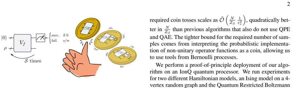
The central object is the quantum coin: a unitary $V_f$ that block-encodes a Hamiltonian function $f[H]$ on a system register and an ancillary register, where measuring the ancillas in the computational basis yields heads if all ancillas are in $|0^a\rangle$. The heads probability is $p_{\mathrm{suc}} = \alpha^2 \mathrm{Tr}[\tilde{f}[H]\rho\tilde{f}[H]^\dagger]$, with $\alpha$ the subnormalization and $\tilde{f}[H]$ the approximate function. For partition-function estimation one takes $\rho$ to be the maximally mixed state and $f[H]=e^{-\beta H/2}$ with $\alpha=e^{-\beta/2}$, so that $p_{\mathrm{suc}} = Z_{\beta}/(e^{\beta} 2^n)$. This identity turns the hard problem of estimating a sum over an exponential number of energy levels into the simple task of estimating the bias of a Bernoulli coin. The coin is implemented either by quantum signal processing or by a variational circuit, and the Bernoulli-process viewpoint is what allows the use of standard tools for binomial proportions and geometric distributions to obtain the sample-complexity bounds.

What would settle it

For a two-qubit Hamiltonian with known eigenbasis, construct an approximate block-encoding whose error matrix is purely off-diagonal in that basis and has spectral norm $\varepsilon'$; then measure the success probability and compare the deviation from the ideal $p_{\mathrm{suc}}$ to the claimed bound $|\tilde{p}_{\mathrm{suc}}-p_{\mathrm{suc}}| \le 3\varepsilon'$. Exceeding that bound would disprove the per-eigenvalue bias analysis.

Watch

Extended reading notes

Core claim

The central claim is that, given a block-encoding of $e^{-\beta H/2}$ with approximation error $\varepsilon'$, the partition function $Z_{\beta} = \mathrm{Tr}[e^{-\beta H}]$ can be estimated to relative error $\varepsilon_r$ and confidence $1-\delta$ by treating the post-selection as a Bernoulli coin. Setting $\rho = 1/2^n$ and $f[H]=e^{-\beta H/2}$ gives $Z_{\beta} = e^{\beta} 2^n p_{\mathrm{suc}}$, where $p_{\mathrm{suc}}$ is the heads probability. Two statistical estimators are proved: one based on the empirical heads fraction (Theorem 1), with sample complexity $O(z_\delta^2 2^n e^{\beta}/(Z_{\beta} \varepsilon_r^2))$, and one based on the number of trials until success (Theorem 3), with average sample complexity $O(2^n e^{\beta}/(\delta \varepsilon_r^2 Z_{\beta}))$. Both scalings are quadratic improvements over the $O((2^n e^{\beta}/Z_{\beta})^2)$ sample complexity of prior Hamiltonian-agnostic algorithms that also do not use QPE or QAE. The proof models the coin tosses as a Bernoulli process and uses binomial-confidence-interval and geometric-distribution analysis; the circuit implementation uses quantum signal processing, whose query complexity per toss is $O(\sqrt{\beta}(\beta+n+\log(1/\varepsilon_r)))$.

Load-bearing premise

The proof that the approximate circuit only changes the success probability by a small amount assumes that the approximation error can be assigned per energy level, but the circuit guarantee is only that the whole matrix is close in the usual matrix sense, so the per-energy-level picture is an extra assumption that the paper does not derive.

Editorial extensions

If this is right

Relative-error sample complexity for partition-function estimation without QPE/QAE becomes $O(2^n e^{\beta}/(Z_{\beta} \varepsilon_r^2))$ instead of the previous $O((2^n e^{\beta}/Z_{\beta})^2 / \varepsilon_r^2)$ scaling.
Because only a block-encoding of $e^{-\beta H/2}$ is required, the algorithm inherits the query complexity of the chosen block-encoding method; with QSP, the total query cost per coin toss is polylogarithmic in the approximation error.
The trials-to-success variant yields a relative-precision estimate without any prior knowledge of $Z_{\beta}$, and its average sample complexity depends on the failure probability only linearly.
The success-probability variant has a milder dependence on confidence (through the normal quantile $z_\delta$) at the cost of setting the block-encoding error to a value that depends on $Z_{\beta}$, which requires a separate relative-error conversion procedure.
The method is naturally compatible with error mitigation by zero-noise extrapolation because the partition function is a single observable expectation; in the 9-qubit proof-of-concept experiment, a simple global-depolarizing noise model suffices to bring the estimates into agreement with exact calculations.

Reading between the lines

Editorial extensions of the paper, not claims the author makes directly.

A rigorous trace-norm argument would likely repair the bias proof in Appendix A, since the bound $|\tilde{p}_{\mathrm{suc}}-p_{\mathrm{suc}}| \le 3\varepsilon'$ can be derived from spectral-norm closeness of the full matrices without assuming per-eigenvalue errors; thus the main conclusion is probably robust to the technical gap in the paper.
The quantum-coin architecture extends beyond partition functions: any normalization constant that can be written as $\mathrm{Tr}[f[H]\rho]$ for a known $\rho$ and a block-encodable $f[H]$ could be sampled in the same way, turning other hard counting problems into single-observable measurements.
The trials-to-success estimator suggests an adaptive protocol that draws coin tosses until a stopping rule is met; since the variance of the geometric distribution is known, one could in principle achieve the same relative error with a data-dependent stopping time that may be smaller in practice.
The noise model used in the experiment assumes a single global depolarizing parameter per layer; testing the same error-mitigation protocol on a device with correlated or non-unital noise would reveal how far the simplicity of the method extends.

Share X Bluesky LinkedIn Reddit HN

Editorial analysis

A structured set of objections, weighed in public.

Desk editor's note, referee report, and a circularity audit.

Desk Editor's Note

read the letter

The core trick is simple: with ρ = I/2^n, the success probability of postselecting a block-encoding of e^{-βH/2} is p_suc = Zβ/(2^n e^β). The paper's real contribution is treating the postselection outcomes as a Bernoulli process and proving sample complexity O(2^n e^β/(Zβ ε_r^2)) for relative-error estimation, quadratically better in 2^n e^β/Zβ than the previous no-QPE/no-QAE algorithms [25,27]. That is a genuine improvement, and the analysis in Theorems 1 and 3 is correct under the ideal-error assumption. The second variant, estimating the mean number of trials to success, is a nice touch because it avoids knowing Zβ a priori, at the cost of a 1/δ dependence instead of log(1/δ).

What it does well: the comparison table is honest, the paper correctly identifies that the identity is elementary and focuses on the estimator analysis, and the QSP cost scaling is stated. The fragmented cooling schedule discussion is thoughtful, noting the open problem of determining a schedule in practice.

The soft spot is real but not fatal. The proof of Theorem 1's bias bound in Eq. (A4) assumes the approximate block-encoding f̃β[H] is diagonal in H's eigenbasis with per-eigenvalue error ε'. Equation (1) only gives spectral-norm closeness of the full matrix, which does not imply commutativity with H. This is a genuine proof gap, but it is repairable: a trace-norm/Hölder argument gives |p̃_suc − p_suc| ≤ 3ε' without needing f̃ to be a function of H, as your stress-test note shows. The central sample-complexity claim survives with a corrected proof, and the paper should add that argument.

Other concerns are minor. Algorithm 1's bias choice requires knowing Zβ; the paper acknowledges this and points to the iterative scheme of [25], but the tight bound is not usable in a single shot. The experimental section is a proof-of-concept on 9 qubits with a variational block-encoding rather than QSP, and it ships no code or data. The single-parameter depolarizing noise model is fitted to one baseline circuit and then applied to all circuits; it works for the few points shown, but this is not systematic validation. I would treat the experiment as a demonstration of the error-mitigation heuristic, not as evidence for the algorithm's scaling.

The citation pattern looks fine; the baseline [27] includes one of the authors, but it is the direct predecessor and the comparison is explicit.

Bottom line: the theoretical result is sound after a proof fix. This paper is for researchers working on partition function estimation, thermal state preparation, and early fault-tolerant algorithms. It deserves a serious referee; I would send it to review with a request to fix the bias proof, ideally by adding the trace-norm argument. I would cite it if I were working on quantum PFE.

Referee Report

1 major / 6 minor

Summary. The manuscript introduces a quantum algorithm for estimating the partition function Z_β = Tr(e^{-βH}) of a bounded-spectrum Hamiltonian H up to relative error, using a "quantum coin toss." The coin is the outcome of a post-selected block-encoding of the imaginary-time propagator e^{-βH/2} applied to the maximally mixed state. The authors propose two estimators: the success-probability (Bernoulli) and the waiting-time (geometric) processes, and prove sample-complexity bounds O(2^n e^β/(Z_β ε_r^2)) for both, claiming a quadratic improvement in 2^n e^β/Z_β over previous no-QPE/no-QAE algorithms. They also provide a QSP implementation cost, a fragmented cooling-schedule variant, and a 9-qubit proof-of-concept experiment on IonQ Aria-1 with variational block-encodings and a simple depolarizing-noise error-mitigation scheme.

Significance. If the results hold, the algorithm is a simple and resource-light approach to partition function estimation, avoiding QPE and QAE, and is well suited to early fault-tolerant hardware. The Bernoulli/geometric analysis is elegant and the practical demonstration with error mitigation is valuable. The central sample-complexity claim is interesting and the comparison with prior work is transparent. However, the proof of Theorem 1 in Appendix A contains a gap that must be repaired; the underlying claim appears correct and the gap is fixable. Overall, this is a worthwhile contribution that requires revision.

major comments (1)

[Appendix A, Eq. (A4)] The bound on |p̃_suc − p_suc| is derived by expanding the trace difference as a sum over eigenvalues of H with a per-eigenvalue error ε'. This step is not justified by the block-encoding condition Eq. (1), which only ensures ||α f̃ − α f|| ≤ ε' in spectral norm for the full operators and does not imply that f̃[H] is diagonal in the eigenbasis of H. The eigenvalue-wise expansion is therefore not a consequence of the stated assumptions. This is load-bearing because Theorem 1's relative-error guarantee and the choice ε' = Z_β/(6 e^β 2^n) ε_r rely on this bound. The claim itself is correct: a trace-norm argument using A = e^{-β/2} f̃ and B = e^{-β/2} f gives |p̃_suc − p_suc| ≤ (1/N)|Tr(A†A − B†B)| ≤ ||A†A − B†B|| ≤ (||A||+||B||)||A−B|| ≤ 3ε', so the theorem remains valid after a corrected proof. The authors should replace the invalid step with such an argument.

minor comments (6)

[Sec. V B] The cooling schedule is defined with β_l = β/2, but the subsequent identity p(Δ_1)...p(Δ_l) = Z_β/(e^β 2^n) is only consistent with β_l = β. Please correct this inconsistency.
[Appendix A 1, Theorem 1] The proof of Theorem 1 uses the Agresti-Coull interval, whose coverage is approximate for finite S. For a formal theorem with confidence 1−δ, the proof should either state the asymptotic nature of the confidence or use a rigorous concentration inequality (e.g., Hoeffding or Chernoff), which would yield the same scaling with slightly changed constants.
[Abstract / Sec. III] The phrase "runtime scaling as O(N/Z_β)" in the abstract refers to the number of coin tosses; the actual runtime also includes the QSP circuit depth O(√β(β+n+log(1/ε_r))) per toss. Please state this distinction explicitly.
[Eq. (A4)] The equation contains typographical errors (e.g., "e−βe−βλ" and malformed exponents) that should be corrected.
[Sec. V C] The variational block-encoding error is reported only as ε' < 10^-2. Reporting the actual trained ε' values per Hamiltonian instance and inverse temperature would allow readers to verify the bias bound used in the main theorems.
[Sec. IV / Fig. 3] The depolarizing-noise strength ξ is fitted with a relative uncertainty over 75%; the paper should note that the agreement in Fig. 3 is qualitative given these uncertainties.

Circularity Check

0 steps flagged · score 0.0 of 10

No significant circularity: Z_beta is obtained from the coin probability by an exact rescaling, and the sample-complexity bounds follow from independent Bernoulli-statistics arguments.

full rationale

The theoretical derivation is self-contained. The coin probability p_suc is defined in Eq. (2) directly from the approximate block-encoding, and Eq. (4) is the exact identity Z_beta = e^beta 2^n p_suc for rho = I/2^n; no free parameter is fitted to Z_beta. The sample-complexity bounds of Theorems 1 and 3 follow from the Agresti-Coull binomial interval and the geometric distribution in Appendix A, and the error budget epsilon' = (1/6)e^beta 2^n epsilon_r is a worst-case bound rather than a fit to the target. The comparison with [25,27] is a baseline, and the fragmented-coin extension cites the authors' own [53] only in an optional refinement, so no load-bearing premise rests on a self-citation. The proof has a genuine but repairable gap: Eq. (A4) assumes the approximate block-encoding is diagonal in H's eigenbasis, which Eq. (1) does not guarantee; a trace-norm argument gives the same order of bias, so the scaling claim is not circularly forced. The experimental noise-model fit at beta* = 0.1 returns the fitted p_suc at that single point by construction, but that point is a demonstration detail and is not an input to the algorithm's complexity claims.

Assumptions & free parameters 1 free parameters · 5 assumptions · 1 invented entities

The theoretical core relies on standard quantum information primitives (block-encoding, QSP) and standard probability inequalities. The experimental section introduces an ad hoc global depolarizing noise model and a variational training assumption. No free parameter is fitted for the theoretical runtime; only the hardware noise strength ξ is fitted. The 'quantum coin' is a definitional device, not a new physical entity.

free parameters (1)

depolarizing noise strength ξ = 0.037 ± 0.028
Fit to nonlinear least squares on the baseline QRBM circuit with identity insertions (Fig. 3a); used to invert the noise channel for all experimental circuits. This parameter does not enter the theoretical runtime but is a fitted quantity in the experimental demonstration.

assumptions (5)

domain assumption Block-encodings and quantum signal processing can implement e^{-βH/2} with spectral-norm error ε' and query complexity O(√β log(1/ε'))
Invoked in Sec. II and Sec. V A when defining the coin and computing gate costs; relies on [36,37,51].
domain assumption The Hamiltonian spectrum can be rescaled to [-1,1] using a known norm bound Λ
Sec. II: 'Assuming the spectrum of H is contained in [-1,1]... One can force it by redefining H → H/Λ with a corresponding rescaling β → Λβ, given an upper bound Λ for the spectral norm of H.'
standard math Standard probability tools: normal-approximation confidence intervals (Agresti-Coull), Chebyshev inequality, geometric distribution
Used in Theorems 1 and 3 and Appendix A to convert samples into relative-error estimates.
ad hoc to paper Global depolarizing noise model with layer-independent strength ξ (Eq. 5)
Assumed in the experimental error-mitigation procedure (Sec. IV, Fig. 2b); not derived from hardware characterization.
ad hoc to paper A hardware-efficient variational ansatz can approximate the block-encoding to ε'<10^-2
Sec. V C: training with COBYLA achieves spectral error below 10^-2 for the instances studied; no guarantee is proven for general Hamiltonians.

invented entities (1)

Quantum coin C(f[H], α, ε', ρ)
purpose: Conceptual device to frame the success/failure of post-selected block-encoding as a Bernoulli random variable
This is a definitional reformulation of a standard postselection measurement, not a new physical entity. It has no falsifiable handle beyond the circuit's success probability.

how reviews work

0 comments

Cite this review

Pith. "Pith review of Partition function estimation with a quantum coin toss." pith.science (2026). https://pith.science/paper/KZSCIBE7

@misc{pith2026241117816,
  author       = {Pith},
  title        = {Pith review of: Partition function estimation with a quantum coin toss},
  year         = {2026},
  howpublished = {\url{https://pith.science/paper/KZSCIBE7}},
  note         = {Machine review of arXiv:2411.17816}
}

abstract

Estimating quantum partition functions is a critical task in a variety of fields. However, the problem is classically intractable in general due to the exponential scaling of the Hamiltonian dimension $N$ in the number of particles. This paper introduces a quantum algorithm for estimating the partition function $Z_\beta$ of a generic Hamiltonian $H$ up to multiplicative error based on a quantum coin toss. The coin is defined by the probability of applying the quantum imaginary-time evolution propagator $f_\beta[H]=e^{-\beta H/{2}}$ at inverse temperature $\beta$ to the maximally mixed state, realized by a block-encoding of $f_\beta[H]$ into a unitary quantum circuit followed by a post-selection measurement. Our algorithm does not use costly subroutines such as quantum phase estimation or amplitude amplification; and the binary nature of the coin allows us to invoke tools from Bernoulli-process analysis to prove a runtime scaling as $\mathcal{O}(N/{Z_\beta})$, quadratically better than previous general-purpose algorithms using similar quantum resources. Moreover, since the coin is defined by a single observable, the method lends itself well to quantum error mitigation. We test this in practice with a proof-of-concept 9-qubit experiment, where we successfully mitigate errors through a simple noise-extrapolation procedure. Our findings offer an interesting alternative for quantum partition function estimation relevant to early-fault quantum hardware.

Figures

Figures reproduced from arXiv: 2411.17816 by the authors.

**Figure 1.** Quantum coin. A quantum-coin toss (relative to an input state ρ) consists of first applying a unitary quantum circuit implementing a block-encoding Vf of the Hamiltonian function f[H] on the system and an ancillary register in a reference state |0⟩ and then measuring the ancillary register in the computational basis. If the ancillary measurement returns 0 (successful post-selection for the correct block of Vf ), we… view at source ↗

**Figure 2.** Variational quantum circuit. (a) The ansatz structure implemented in the IonQ’s Aria-1 machine. Purple circles represent GPI2(ϕ) gates, and the blue box represent MS(ϕ1, ϕ2, θ) gates. (b) Noise model used for error mitigation. We assume the hardware implements each ideal layer W(θj ), followed by a global depolarizing channel Λξ. Identities in the form of 1 = W(θ ′ )W† (θ ′ ) are inserted to increase the noise stre… view at source ↗

**Figure 3.** Experimental results. (a) Noise strength determination using identity insertion. The plot shows the empirical value over 3000 shots of the success probability for different numbers of layers (circuit depths) for fixed H and β ∗ = 0.1. The dashed line shows the fit of Eq. (6) which gives ξ = 0.037 ± 0.028 and pˆ (β ∗) suc = 0.38 ± 0.05. The uncertainties associated with ξ and p (β ∗) suc are the standard deviations a… view at source ↗

Discussion (0). Continue with ORCID to comment.

Reference graph

Works this paper leans on

66 extracted references · 55 canonical work pages

[25]

˜O N Zβ 2 e2β22a ε2r (β2 +n2) 2a + 1 – any block-encoding of H

work page
[27]

heads” if 4 the measurement returns only zeros and “tails

˜O e2βN2 ε2r Z2β √β a + 1 – any block-encoding of H this work ˜O N Zβ eβ ε2r a – any block-encoding of e−βH this work + QSP ˜O N Zβ eβ ε2r √β a – any block-encoding of H Table I. Overview of quantum algorithms for PFE. Comparison in terms of runtime, number of ancillas, subroutines required, type of Hamiltonian supported, and the access model – i.e., a qu...

work page
[1]

Huang, Statistical Mechanics, 2nd edition (Wiley, 1987)

K. Huang, Statistical Mechanics, 2nd edition (Wiley, 1987)

work page 1987
[2]

tails”; 4 while c ̸= “heads

We note that, to our convenience, zδ is an extremely slow-growing function of the confidence. For instance, z.05 = 1.96, while z10−9 = 6.11. Theorem 1 (PFE using the success probability) . Given a quantum coin C fβ[H], e−β/2, ε′, 1/2n), with approxima- tion error ε′ ≤ Zβ 6 eβ 2n εr, the partition function of H at in- verse temperature β can be estimated u...

work page
[3]

E. Freire, Statistical thermodynamic analysis of differential scanning calorimetry data: Structural deconvolution of heat capacity function of proteins, in Part B: Numerical Computer Methods, Methods in Enzymology, V ol. 240 (Academic Press,

work page
[4]

Zwanzig, Two-state models of protein folding kinetics, Proc Natl Acad Sci U S A 94, 148 (1997)

R. Zwanzig, Two-state models of protein folding kinetics, Proc Natl Acad Sci U S A 94, 148 (1997)

work page 1997
[5]

Friedman, Inferring cellular networks using probabilistic graphical models, Science 303, 799 (2004)

N. Friedman, Inferring cellular networks using probabilistic graphical models, Science 303, 799 (2004)

work page 2004
[6]

H. GM, M. K. Gourisaria, M. Pandey, and S. S. Rautaray, 11 A comprehensive survey and analysis of generative models in machine learning, Computer Science Review 38, 100285 (2020)

work page 2020

Show all 66 references

[7]

Koller and N

D. Koller and N. Friedman, Probabilistic Graphical Models: Principles and Techniques - Adaptive Computation and Ma- chine Learning (The MIT Press, 2009)

2009
[8]

P. M. Long and R. A. Servedio, Restricted boltzmann ma- chines are hard to approximately evaluate or simulate, in Pro- ceedings of the 27th International Conference on Interna- tional Conference on Machine Learning , ICML’10 (Omni- press, Madison, WI, USA, 2010) p. 703–710

2010
[9]

Jerrum and A

M. Jerrum and A. Sinclair, Polynomial-time approximation al- gorithms for the ising model, SIAM Journal on Computing22, 1087 (1993), https://doi.org/10.1137/0222066

1993 doi
[10]

L. Stockmeyer, The complexity of approximate counting, in Proceedings of the Fifteenth Annual ACM Symposium on The- ory of Computing, STOC ’83 (Association for Computing Ma- chinery, 1983) p. 118

1983
[11]

O 1 εr q N Zβ (β + log1 εr ) a +O log 1 εr QAE H ≥ 0 block-encoding ofH′ (effective√H )
[12]

Banks, J

J. Banks, J. Garza-Vargas, A. Kulkarni, and N. Srivastava, Pseudospectral shattering, the sign function, and diagonaliza- tion in nearly matrix multiplication time, Foundations of com- putational mathematics 23, 1959 (2023)

2023
[13]

Weiße, G

A. Weiße, G. Wellein, A. Alvermann, and H. Fehske, The kernel polynomial method, Reviews of Modern Physics 78, 275–306 (2006)

2006
[14]

Istrail, Statistical mechanics, three-dimensionality and np- completeness: I

S. Istrail, Statistical mechanics, three-dimensionality and np- completeness: I. universality of intracatability for the partition function of the ising model across non-planar surfaces (ex- tended abstract), in Proceedings of the Thirty-Second Annual ACM Symposium on Theory o...

2000
[15]

D. Weitz, Counting independent sets up to the tree threshold, in Proceedings of the Thirty-Eighth Annual ACM Symposium on Theory of Computing, STOC ’06 (Association for Comput- ing Machinery, New York, NY , USA, 2006) p. 140–149

2006
[16]

Bulatov and M

A. Bulatov and M. Grohe, The complexity of partition func- tions, Theoretical Computer Science 348, 148 (2005)

2005
[17]

Barvinok and N

A. Barvinok and N. Barvinok, More on zeros and approxi- mation of the ising partition function, Forum of Mathematics, Sigma 9, e46 (2021)

2021
[18]

Bravyi, A

S. Bravyi, A. Chowdhury, D. Gosset, and P. Wocjan, Quan- tum hamiltonian complexity in thermal equilibrium, Nature Physics 18, 1367–1370 (2022)

2022
[19]

A. W. Harrow, S. Mehraban, and M. Soleimanifar, Classical algorithms, correlation decay, and complex zeros of partition functions of quantum many-body systems, in Proceedings of the 52nd Annual ACM SIGACT Symposium on Theory of Com- puting, STOC ’20 (ACM, 2020)

2020
[20]

Wocjan, C.-F

P. Wocjan, C.-F. Chiang, D. Nagaj, and A. Abeyesinghe, Quantum algorithm for approximating partition functions, Phys. Rev. A 80, 022340 (2009)

2009
[21]

Montanaro, Quantum speedup of monte carlo methods, Proceedings of the Royal Society A: Mathematical, Physical and Engineering Sciences 471, 20150301 (2015)

A. Montanaro, Quantum speedup of monte carlo methods, Proceedings of the Royal Society A: Mathematical, Physical and Engineering Sciences 471, 20150301 (2015)

2015
[22]

A. W. Harrow and A. Y . Wei, Adaptive quantum simulated an- nealing for bayesian inference and estimating partition func- tions, in Proceedings of the Fourteenth Annual ACM-SIAM Symposium on Discrete Algorithms(Society for Industrial and Applied Mathematics, 2020) p. 193–212

2020
[23]

Sinclair, P

A. Sinclair, P. Srivastava, and M. Thurley, Approximation algorithms for two-state anti-ferromagnetic spin systems on bounded degree graphs, Journal of Statistical Physics 155 (2014)

2014
[24]

˜O q N Zβ β5 ε2r a +O n +β log β εr QPE, QAA, QAE, cooling schedule quantum H ≥ 0 e−itH [20–23] ˜O n√τ εr a +O logτ log 1 εr QAE, QPE, cooling schedule classical H ≥ 0 Markov chain quantum walk with relaxation timeτ
[26]

A. M. Alhambra, Quantum many-body systems in thermal equilibrium, PRX Quantum 4, 040201 (2023)

2023
[28]

A. Y . Kitaev, Quantum measurements and the abelian stabi- lizer problem (1995), arXiv:quant-ph/9511026

1995 arXiv
[29]

Brassard, P

G. Brassard, P. Høyer, M. Mosca, and A. Tapp, Quantum am- plitude amplification and estimation, Quantum Computation and Information , 53–74 (2002)

2002
[30]

O 1 ε2r χ exp h 2β m (1−χ)2m−1 i O(1) – mlocal termshj κ = Pm j=1∥hj∥ implementation of eachhj
[31]

˜O n3 ε2r a +O(1) Cooling schedule, β ≤ 1 615DJ, J = hkl k-local termshj, ∥hj∥ ≤h, each qubit inl′ < lterms block-encoding ofH
[32]

Arunachalam, V

S. Arunachalam, V . Havlicek, G. Nannicini, K. Temme, and P. Wocjan, Simpler (classical) and faster (quantum) algorithms for gibbs partition functions, Quantum 6, 789 (2022)

2022
[33]

Poulin and P

D. Poulin and P. Wocjan, Sampling from the thermal quantum gibbs state and evaluating partition functions with a quantum computer, Phys. Rev. Lett.103, 220502 (2009)

2009
[34]

A. N. Chowdhury, R. D. Somma, and Y . Subasi, Computing partition functions in the one clean qubit model, Physical Re- view A 103, 032422 (2021), arXiv:1910.11842 [quant-ph]

2021 arXiv
[35]

Jackson, T

A. Jackson, T. Kapourniotis, and A. Datta, Partition-function estimation: Quantum and quantum-inspired algorithms, Phys- ical Review A 107, 10.1103/physreva.107.012421 (2023)

2023 doi
[36]

Tosta, T

A. Tosta, T. de Lima Silva, G. Camilo, and L. Aolita, Random- ized semi-quantum matrix processing, npj Quantum Inf10, 93 (2024)

2024
[37]

Zhang, J

D. Zhang, J. L. Bosse, and T. Cubitt, Dissipative quantum gibbs sampling (2023), arXiv:2304.04526 [quant-ph]

2023 arXiv
[38]

Rouz ´e, D

C. Rouz ´e, D. S. Franc ¸a, and ´Alvaro M. Alhambra, Opti- mal quantum algorithm for gibbs state preparation (2024), arXiv:2411.04885 [quant-ph]

2024
[39]

Wu and J

Y . Wu and J. B. Wang, Estimating gibbs partition function with quantum clifford sampling, Quantum Science and Tech- nology 7, 025006 (2022)

2022
[40]

Matsumoto, Y

K. Matsumoto, Y . Shingu, S. Endo, S. Kawabata, S. Watabe, T. Nikuni, H. Hakoshima, and Y . Matsuzaki, Calculation of gibbs partition function with imaginary time evolution on near-term quantum computers, Japanese Journal of Applied Physics 61, 042002 (2022)

2022
[41]

Lemieux, B

J. Lemieux, B. Heim, D. Poulin, K. Svore, and M. Troyer, Efficient Quantum Walk Circuits for Metropolis-Hastings Al- gorithm, Quantum 4, 287 (2020)

2020
[42]

Wocjan and K

P. Wocjan and K. Temme, Szegedy walk unitaries for quan- tum maps, Communications in Mathematical Physics 402, 3201–3231 (2023)

2023
[43]

G. H. Low and I. L. Chuang, Hamiltonian Simulation by Qubitization, Quantum 3, 163 (2019)

2019
[44]

Gily ´en, Y

A. Gily ´en, Y . Su, G. H. Low, and N. Wiebe, Quantum sin- gular value transformation and beyond: Exponential improve- 12 ments for quantum matrix arithmetics, in Proceedings of the 51st Annual ACM SIGACT Symposium on Theory of Comput- ing, STOC 2019 (Association for Computing...

2019
[45]

de Lima Silva, L

T. de Lima Silva, L. Borges, and L. Aolita, Fourier-based quantum signal processing (2022), arXiv:2206.02826 [quant- ph]

2022 arXiv
[46]

Y . Dong, L. Lin, and Y . Tong, Ground-state preparation and energy estimation on early fault-tolerant quantum computers via quantum eigenvalue transformation of unitary matrices, PRX Quantum 3, 10.1103/prxquantum.3.040305 (2022)

2022 doi
[47]

R. G. Melko, G. Carleo, J. Carrasquilla, and J. I. Cirac, Restricted boltzmann machines in quantum physics, Nature Physics 15, 887 (2029)
[48]

A. N. Chowdhury and R. D. Somma, Quantum algorithms for gibbs sampling and hitting-time estimation, Quantum Info. Comput. 17, 41–64 (2017)

2017
[49]

F. G. S. L. Brandao, Entanglement theory and the quantum simulation of many-body physics (2008), arXiv:0810.0026 [quant-ph]

2008 arXiv
[50]

L. D. Brown, T. T. Cai, and A. DasGupta, Interval Estimation for a Binomial Proportion, Statistical Science 16, 101 (2001)

2001
[51]

A. M. Pires and C. Amado, Interval estimators for a bino- mial proportion: Comparison of twenty methods, REVSTAT- Statistical Journal 6, 165 (2008)

2008
[52]

Kikuchi, C

Y . Kikuchi, C. Mc Keever, L. Coopmans, M. Lubasch, and M. Benedetti, Realization of quantum signal processing on a noisy quantum computer, npj Quantum Information 9, 10.1038/s41534-023-00762-0 (2023)

2023 doi
[53]

Temme, S

K. Temme, S. Bravyi, and J. M. Gambetta, Error mitigation for short-depth quantum circuits, Phys. Rev. Lett.119, 180509 (2017)

2017
[54]

Li and S

Y . Li and S. C. Benjamin, Efficient variational quantum simu- lator incorporating active error minimization, Phys. Rev. X 7, 021050 (2017)

2017
[55]

K. W. Vugrin, L. P. Swiler, R. M. Roberts, N. J. Stucky-Mack, and S. P. Sullivan, Confidence region estimation techniques for nonlinear regression in groundwater flow: Three case stud- ies, Water Resources Research 43, W03423 (2007)

2007
[56]

Ku, Notes on the use of propagation of error formulas, Jour- nal of Research of the National Bureau of Standards, Section C: Engineering and Instrumentation 70C, 263 (1966)

H. Ku, Notes on the use of propagation of error formulas, Jour- nal of Research of the National Bureau of Standards, Section C: Engineering and Instrumentation 70C, 263 (1966)

1966
[57]

V ovrosh, K

J. V ovrosh, K. E. Khosla, S. Greenaway, C. Self, M. S. Kim, and J. Knolle, Simple mitigation of global depolarizing errors in quantum simulations, Phys. Rev. E 104, 035309 (2021)

2021
[58]

Sachdeva and N

S. Sachdeva and N. Vishnoi, Approximation Theory and the Design of Fast Algorithms (2013), arXiv:1309.4882 [cs, math]

2013 arXiv
[59]

R. D. Somma, S. Boixo, H. Barnum, and E. Knill, Quantum simulations of classical annealing processes, Physical Review Letters 101, 10.1103/physrevlett.101.130504 (2008)

2008 doi
[60]

T. L. Silva, M. M. Taddei, S. Carrazza, and L. Aolita, Frag- mented imaginary-time evolution for early-stage quantum sig- nal processors, Scientific Reports 13, 18258 (2023)

2023
[61]

Getting started with Native Gates, https://ionq.com/ docs/getting-started-with-native-gates , ac- cessed: 2023-08-20

2023
[62]

G. Wang, D. S. Franc ¸a, G. Rendon, and P. D. Johnson, Faster ground state energy estimation on early fault-tolerant quantum computers via rejection sampling (2023), arXiv:2304.09827 [quant-ph]. Appendix A: Proofs of theorems and lemmas

2023 arXiv
[63]

Proof of Theorem 1 Suppose that of the total number of coin flips,Ssuc of them were successes. Agresti-Coull interval [43] can be used to obtain an estimate for the probability of the coin as ˆp(β) suc = 1 S + z2 δ Ssuc + z2 δ 2 (A1) up to an additive error εp ≤ zδ s ˆp(β) suc...
[64]

For instance, z.05 = 1.96, while z10−9 = 6.11

zδ is a slow-varying function of the confidence. For instance, z.05 = 1.96, while z10−9 = 6.11. From the success probability estimate, an estimate for the partition function is obtained using Eq. (4). The choice of precision εp ≤ Zβ 2neβ εr 2 ensures a target relative precisio...
[65]

Therefore, the average number of repetitions to get one success is ¯R = ∞X r=1 p(β) suc (1 − p(β) suc )r−1 r = 1 p(β) suc , (A5) by using that (1 − x)−1 = P∞ r=0 xr

Proof of Lemma 2 The probability that a success will occur only in the R-th run of the circuit is given as Pr (R) = (1 − p(β) suc )R−1p(β) suc , which is the probability of getting R − 1 consecutive failures times the probability of obtaining one success. Therefore, the averag...
[66]

One can show that R2 = ∞X r=1 p(β) suc (1 − p(β) suc )r−1 r2 = 2 − p(β) suc p(β) suc 2

Proof of Theorem 3 Proof. One can show that R2 = ∞X r=1 p(β) suc (1 − p(β) suc )r−1 r2 = 2 − p(β) suc p(β) suc 2 . (A6) Combining the above with Eq. (A5) gives the variance Var(R) = R2 − ¯R2 = 1 − p(β) suc p(β) suc 2 . (A7) Chebyshev inequality then yields the number of sample...

Pith tools

Reviewed August 12, 2026 · model on record in the stance chip above.

[1] [25]

˜O N Zβ 2 e2β22a ε2r (β2 +n2) 2a + 1 – any block-encoding of H

work page

[2] [27]

heads” if 4 the measurement returns only zeros and “tails

˜O e2βN2 ε2r Z2β √β a + 1 – any block-encoding of H this work ˜O N Zβ eβ ε2r a – any block-encoding of e−βH this work + QSP ˜O N Zβ eβ ε2r √β a – any block-encoding of H Table I. Overview of quantum algorithms for PFE. Comparison in terms of runtime, number of ancillas, subroutines required, type of Hamiltonian supported, and the access model – i.e., a qu...

work page

[3] [1]

Huang, Statistical Mechanics, 2nd edition (Wiley, 1987)

K. Huang, Statistical Mechanics, 2nd edition (Wiley, 1987)

work page 1987

[4] [2]

tails”; 4 while c ̸= “heads

We note that, to our convenience, zδ is an extremely slow-growing function of the confidence. For instance, z.05 = 1.96, while z10−9 = 6.11. Theorem 1 (PFE using the success probability) . Given a quantum coin C fβ[H], e−β/2, ε′, 1/2n), with approxima- tion error ε′ ≤ Zβ 6 eβ 2n εr, the partition function of H at in- verse temperature β can be estimated u...

work page

[5] [3]

E. Freire, Statistical thermodynamic analysis of differential scanning calorimetry data: Structural deconvolution of heat capacity function of proteins, in Part B: Numerical Computer Methods, Methods in Enzymology, V ol. 240 (Academic Press,

work page

[6] [4]

Zwanzig, Two-state models of protein folding kinetics, Proc Natl Acad Sci U S A 94, 148 (1997)

R. Zwanzig, Two-state models of protein folding kinetics, Proc Natl Acad Sci U S A 94, 148 (1997)

work page 1997

[7] [5]

Friedman, Inferring cellular networks using probabilistic graphical models, Science 303, 799 (2004)

N. Friedman, Inferring cellular networks using probabilistic graphical models, Science 303, 799 (2004)

work page 2004

[8] [6]

H. GM, M. K. Gourisaria, M. Pandey, and S. S. Rautaray, 11 A comprehensive survey and analysis of generative models in machine learning, Computer Science Review 38, 100285 (2020)

work page 2020