REVIEW 3 major objections 5 minor 37 references
Multi-Frequency Models of Black Hole Photon Rings from Low-Luminosity Accretion Disks
T0 review · 3 major / 5 minor · reviewed 2026-08-12 · deepseek-v4-flash
Pith's one-line read The apparent radius of a black hole's photon ring shifts with frequency in a way that exposes electron temperature at low frequencies and magnetic field strength at high frequencies.
desk verdict Useful fast modeling tool with a careful resolution study, but the magnetic-field inference in the abstract is stronger than the parameter study actually supports. read the letter →
The pith
A machine-rendered reading of the paper's core claim, the machinery that carries it, and where it could break.
The reading
What carries the argument
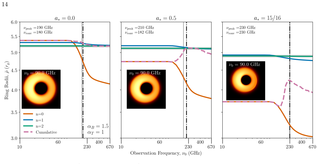
The engine is an analytic solution of the relativistic radiative transfer equation in which synchrotron emission and absorption coefficients are held constant on each geodesic pass through an equatorial disk, giving each sub-image intensity $I_{\nu_0,n} = S_{\nu,n}(1-e^{-\tau_{\nu,n}})$ with the optical depth of earlier passes suppressing later ones (Eqs. 5-6). The disk is a three-power-law model for electron density, temperature, and magnetic field calibrated to M87*, with density normalized so the 230 GHz flux is 0.5 Jy. The Adaptive Analytical Ray Tracing (AART) code supplies the analytic photon geodesics and adaptive image grids, and the ring radius is defined as the peak of the radial intensity slice at each position angle, averaged through the second-moment method of Chael et al. 2021. The load-bearing metric is the convergence frequency $\nu_{\rm conv}$, defined as the frequency where the cumulative image radius comes within 2% of the $n=2$ radius (or, failing that, reaches its closest approach), which marks the onset of photon-ring visibility.
What would settle it
Ray-trace a vertically resolved GRMHD simulation of M87* with a continuous radiative-transfer solver at 90, 230, and 350 GHz and measure the brightness-peak radius at each frequency; if the radius does not stop shrinking with the temperature index at low frequency and start following the magnetic field at high frequency in the model's predicted order, the central claim fails. An observational counterpart would be matched 86/230/345 GHz images of M87*: the model predicts a nearly constant ring radius below the transition and a shrinking radius above it.
Extended reading notes
Core claim
The paper's central claim is that the image-domain radius of the $n=0$ direct image and the visibility of the $n=1,2$ photon rings vary with observing frequency in a parameter-dependent way that can be inverted to infer plasma properties. At low frequencies, where the disk is optically thick, the brightness peak sits where the redshifted electron temperature is highest, so the ring radius is controlled by the temperature normalization $T_{e,0}$ and index $\alpha_T$. At higher frequencies, where the disk becomes optically thin, the peak tracks the radius where the synchrotron critical frequency equals the emitted frequency, which depends on magnetic field strength, so the magnetic index $\alpha_B$ dominates. A secondary claim is that the cumulative image's brightest point can jump between the $n=0$ and $n=2$ rings depending on spin, inclination, and position angle, so any single image-domain ring radius must be defined and interpreted carefully.
Load-bearing premise
The load-bearing assumption is that the synchrotron emission and absorption coefficients are constant along each pass through a thin disk of fixed opening angle $h/r=0.5$; real accretion disks have gradients along the ray path, and if those gradients are strong, the predicted ring radii and transition frequencies will shift.
Editorial extensions
If this is right
- At frequencies where the disk is optically thick, measuring the ring radius gives a direct read on the electron temperature profile; steeper temperature falloff yields a smaller halo.
- At optically thin frequencies, the radius becomes a probe of magnetic field strength, so pairing low- and high-frequency images breaks the degeneracy between temperature and field parameters.
- The convergence frequency $\nu_{\rm conv}$ and the spectral peak frequency $\nu_{\rm peak}$ agree within roughly 50 GHz for most studied M87*-like models, so an SED peak can budget when higher-order photon rings start to matter.
- The $n=1$ and $n=2$ ring radii track the critical curve and depend mainly on spin and inclination, preserving photon rings as a mostly gravitational observable even as the $n=0$ image carries the plasma information.
- Because the brightest ring can switch between $n=0$ and $n=2$ across the image for high spin, radius measurements in the image domain need explicit definitions; visibility-domain analysis may be a cleaner route.
Reading between the lines
- The authors leave implicit that the analytic model could serve as a fast likelihood surrogate for GRMHD parameter estimation, since it explores a much larger parameter space at far lower cost than full simulations.
- If the radius ordering holds, simultaneous EHT/BHEX observations at 86, 230, and 345 GHz could be interpreted as a two-band plasma thermometer and magnetometer, giving an empirical handle on $T_e$ and $B$ without polarimetric modeling.
- A testable consequence the paper does not pursue: $\nu_{\rm conv}$ should move with accretion state, since hotter models shift both $\nu_{\rm peak}$ and $\nu_{\rm conv}$ downward; time monitoring of M87* could check whether the ring radius at a fixed frequency tracks the SED's peak.
- The constant-coefficient-per-pass assumption could be checked by full GRMHD ray tracing; if vertical gradients shift the predicted radii by more than the quoted convergence, the clean temperature versus magnetic field separation would need revision.
Editorial analysis
A structured set of objections, weighed in public.
Referee Report
Summary. The paper introduces an astrophysically motivated synchrotron emission model for the AART ray-tracing code, enabling fast multi-frequency (10–670 GHz) images of black hole accretion disks. The model treats emission and absorption as constant on each disk crossing, adopts power-law radial profiles for density, temperature, and magnetic field, and normalizes each model to a 230 GHz flux of 0.5 Jy, matching M87*. The authors compute flux densities, image-domain ring radii, and optical depths for a parameter grid in α_T, α_B, T_e,0, and spin. They define a convergence frequency ν_conv marking when the cumulative image radius approaches the n=2 photon ring, compare it to the SED peak, and show that higher-order rings are largely geometry-dominated while the n=0 image depends on plasma parameters. The central claim is that low-frequency ring radii are set by electron temperature, while higher-frequency radii are set by magnetic field strength, enabling inference of plasma parameters from multi-frequency observations. The paper also demonstrates time-variable and blurred images using Gaussian random fields.
Significance. If the central dichotomy holds, this is a valuable fast, open-source tool for interpreting upcoming multi-frequency EHT and BHEX observations and for forecasting when photon rings become visible. The paper ships publicly available code, uses standard synchrotron radiative transfer, and includes a careful resolution study (Appendix B), all of which are strengths. The qualitative result that n=1 and n=2 radii are geometry-dominated while the n=0 image is astrophysics-dominated is well supported. The specific inference claim—that the low-frequency radius probes electron temperature and the high-frequency radius probes magnetic field strength—is interesting and potentially impactful, but, as detailed below, the current parameter study does not cleanly demonstrate the magnetic-field part of that claim.
major comments (3)
- [Abstract, §3.2.1, §5, Table 1] The central claim that ring radii are set by electron temperature at low frequencies and by magnetic field strength at high frequencies is not fully supported by the parameter study. In Table 1, the magnetic field normalization B0 is fixed at 8 G; only the radial power-law index αB is varied. Because B enters the synchrotron coefficients only through νc ∝ B Θe^2 (Eq. 14), varying αB changes the radial profile of emission but does not probe the field amplitude at the anchor radius. Moreover, Appendix A normalizes each model by rescaling n_th,0 to force F230 = 0.5 Jy; since n_th,0 also sets the optical-depth scale, an independent change in B0 (or T_e,0) would be partially absorbed into the density normalization and would shift νconv. The quoted temperature-vs-magnetic-field dichotomy is therefore demonstrated only for the profile index αB with B0 fixed, not for the field strength B0 that the abstract and conclusions invoke. I request that the authors either vary B0 (and show whether the effect survives the 0.5 Jy renormalization) or explicitly rephrase the claim to refer to the radial profile index αB.
- [§2.1, Eqs. (5)–(9), Table 1] The analytic radiative transfer solution assumes jν and κν are constant on each pass through the disk, and the vertical structure is reduced to a fixed opening angle θdisk = h/r = 0.5 (Eq. 8). These assumptions are acknowledged as simplifying, but they are load-bearing for the reported radii, optical depths, and νconv values. Realistic flows exhibit gradients along the raypath and height ratios that vary with radius and magnetization; the quantitative values in Figs. 7–9 and the relative ordering of νconv and νpeak could shift if θdisk were different or if jν and κν were integrated in sub-steps across the disk thickness. I ask for a sensitivity test—for example, recomputing a fiducial model with θdisk = 0.3 and 0.7, or splitting each disk crossing into several integration steps—to confirm that the qualitative temperature-vs-field dichotomy is not an artifact of this vertical-structure approximation.
- [§3.4 and Fig. 11] The definition of νconv as the image-domain transition frequency is clear, but the paper also calls it 'the transition to the optically thin regime.' Fig. 11 shows that the intensity-weighted optical depth equals unity only at frequencies above both νconv and νpeak for the models shown. This is not necessarily an error, but the terminology is misleading: νconv marks when the cumulative image radius approaches the n=2 ring, which depends on relative brightness and image structure, not on the physical criterion ⟨τ⟩ = 1. I recommend rephrasing to distinguish the image-domain convergence frequency from the physical optical-depth transition throughout the text.
minor comments (5)
- [§5] In the concluding paragraph, 'the the magnetic field strength' contains a duplicated article; please correct to 'the magnetic field strength.'
- [Figs. 12 and 13] The captions for Figs. 12 and 13 state 'a∗ = 15/26', while the text and Table 1 use a∗ = 15/16. Please correct this typo if the intended spin is 15/16.
- [Fig. 12 caption] The caption lists blurring kernels θblur = [0, 1, 5, 10] μas and then associates them with 'Earth to L2, Earth to Moon, GEO, LEO' baselines, but the order is ambiguous (0 μas is the unblurred image, not a baseline). Please clarify which kernel corresponds to which baseline configuration.
- [Eq. (24)] The exponent 'n1/2 scale' is unclear in the printed text; please typeset it as nscale^{1/2} or otherwise define the quantity explicitly.
- [Appendix B and Fig. 15] Appendix B states that at 8000×8000 pixels the cumulative radius 'has not become completely independent of resolution,' while the Fig. 15 caption says the same resolution is 'well within the range of being safely independent.' Please harmonize the wording to avoid an apparent contradiction.
Circularity Check
No significant circularity: multi-frequency ring radii are forward-model outputs from stated radiative-transfer assumptions; flux normalization is calibration, not a predicted result.
full rationale
The paper builds an analytic synchrotron/thermal disk model and ray-traces it; the reported ring radii, νconv, and νpeak are all computed from the model, not fitted to the quantities they are used to infer. The low-frequency temperature control follows directly from the Planck source function (Eq. 17) in the optically thick limit, and the high-frequency magnetic-field dependence enters through νc ∝ BΘ_e^2 in the emission and absorption coefficients (Eqs. 13-14). Because these are stated model assumptions, the conclusions are self-consistent forward-model results, not circular reductions. The density normalization nth,0 is chosen to match F230 = 0.5 Jy (Appendix A), and Te,0 is chosen to put the SED peak near 230 GHz; this calibrates the absolute flux scale, but the frequency-dependent radius curves are not statistically forced by this calibration, since uniform density scaling does not change the peak radius of the n=0 image, and radius transitions are governed by the optical depth profile rather than by total flux. Self-citations to AART and earlier photon-ring work are methodological references, not load-bearing uniqueness or ansatz claims. The overstatement that 'magnetic field strength' dominates when only αB (not B0) was varied is a scope limitation, not circularity; likewise the proximity of νconv to νpeak reflects both metrics tracking the same τ≈1 transition, which the paper explicitly acknowledges. No step reduces an output to a fitted input or to a self-citation.
Assumptions & free parameters
free parameters (8)
- nth,0 (electron density normalization at Rb) =
2.8e3 to 4e6 cm^-3 depending on model, mean 4e5
- Te,0 (electron temperature at Rb) =
[3, 5, 7] x 10^10 K; fiducial 3 x 10^10 K
- B0 (magnetic field strength at Rb) =
8 Gauss
- alpha_n (density power-law index) =
0.7
- alpha_T (temperature power-law index) =
[1.5, 1, 0.5]
- alpha_B (magnetic field power-law index) =
[2, 1.5, 1]
- theta_disk (disk opening angle h/r) =
0.5
- Rb (power-law normalization radius) =
5 rg
assumptions (6)
- standard math Kerr metric and null geodesic equations are exact, and AART traces photon paths analytically.
- domain assumption Thermal synchrotron emissivity and absorption from Dexter (2016), with a Planck source function, describe the disk radiation.
- ad hoc to paper Emission and absorption coefficients are constant on each geodesic pass through the disk.
- ad hoc to paper Disk density, temperature, and magnetic field follow power laws anchored at Rb = 5 rg.
- domain assumption The flow follows the Cunningham Keplerian model with four-velocity parameters set to unity.
- domain assumption No jet, no non-thermal electrons, no scattering, and no emission outside the equatorial disk.
Cite this review
Pith. "Pith review of Multi-Frequency Models of Black Hole Photon Rings from Low-Luminosity Accretion Disks." pith.science (2026). https://pith.science/paper/2ADJRJ33
@misc{pith2026241117884,
  author       = {Pith},
  title        = {Pith review of: Multi-Frequency Models of Black Hole Photon Rings from Low-Luminosity Accretion Disks},
  year         = {2026},
  howpublished = {\url{https://pith.science/paper/2ADJRJ33}},
  note         = {Machine review of arXiv:2411.17884}
}
read the original abstract
Images of black holes encode both astrophysical and gravitational properties. Detecting highly-lensed features in images can differentiate between these two effects. We present an accretion disk emission model coupled to the Adaptive Analytical Ray Tracing (AART) code that allows a fast parameter space exploration of black hole photon ring images produced from synchrotron emission from 10 to 670 GHz. As an application, we systematically study several disk models and compute their total flux density, average radii, and optical depth. The model parameters are chosen around fiducial values calibrated to general relativistic magnetohydrodynamic (GRMHD) simulations and observations of M87*. For the parameter space studied, we characterize the transition between optically thin and thick regimes and the frequency at which the first photon ring is observable. Our results highlight the need for careful definitions of photon ring radius in the image domain, as in certain models, the highly lensed photon ring is dimmer than the direct emission at certain angles. We find that at low frequencies, the ring radii are set by the electron temperature, while at higher frequencies, the magnetic field strength plays a more significant role, demonstrating how multi-frequency analysis can also be used to infer plasma parameters. Lastly, we show how our implementation can qualitatively reproduce multifrequency black hole images from GRMHD simulations when adding time-variability to our disk model through Gaussian random fields. This approach provides a new method for simulating observations from the Event Horizon Telescope (EHT) and the proposed Black Hole Explorer (BHEX) space mission.
Figures


Figures from the paper (12 more)




Reference graph
Works this paper leans on
-
[1]
Astropy Collaboration, Robitaille, T. P., Tollerud, E. J., et al. 2013, A&A, 558, A33, doi: 10.1051/0004-6361/201322068 Astropy Collaboration, Price-Whelan, A. M., Sip˝ ocz, B. M., et al. 2018, AJ, 156, 123, doi: 10.3847/1538-3881/aabc4f Astropy Collaboration, Price-Whelan, A. M., Lim, P. L., et al. 2022, ApJ, 935, 167, doi: 10.3847/1538-4357/ac7c74
-
[2]
Bardeen, J. M. 1974, Symposium - International Astronomical Union, 64, 132–144, doi: 10.1017/s0074180900236218
-
[3]
Broderick, A. E., Fish, V. L., Doeleman, S. S., & Loeb, A. 2011, The Astrophysical Journal, 735, 110, doi: 10.1088/0004-637x/735/2/110
-
[4]
Broderick, A. E., & Loeb, A. 2006, MNRAS, 367, 905, doi: 10.1111/j.1365-2966.2006.10152.x —. 2009, ApJ, 697, 1164, doi: 10.1088/0004-637X/697/2/1164 C´ ardenas-Avenda˜ no, A., & Held, A. 2024, Phys. Rev. D, 109, 064052, doi: 10.1103/PhysRevD.109.064052 C´ ardenas-Avenda˜ no, A., Keeble, L., & Lupsasca, A. 2024, Phys. Rev. D, 109, 124052, doi: 10.1103/Phys...
arXiv 2006
-
[5]
Chael, A., Issaoun, S., Pesce, D. W., et al. 2023, The Astrophysical Journal, 945, 40, doi: 10.3847/1538-4357/acb7e4
-
[6]
Chael, A., Johnson, M. D., & Lupsasca, A. 2021, The Astrophysical Journal, 918, 6, doi: 10.3847/1538-4357/ac09ee 23
-
[7]
Chael, A., Narayan, R., & Johnson, M. D. 2019, MNRAS, 486, 2873, doi: 10.1093/mnras/stz988
-
[8]
Chang, D. O., Johnson, M. D., Tiede, P., & Palumbo, D. C. M. 2024, Astrophys. J., 974, 143, doi: 10.3847/1538-4357/ad6b28
Show all 37 references
-
[9]
Cunningham, C. T. 1975, ApJ, 202, 788, doi: 10.1086/154033
1975 doi
-
[10]
2024, AstroModels: Code for Multi-frequency Models of Black Hole Photon Rings, doi: 10.5281/zenodo.14629536
Desire, T., C´ ardenas-Avenda˜ no, A., & Chael, A. 2024, AstroModels: Code for Multi-frequency Models of Black Hole Photon Rings, doi: 10.5281/zenodo.14629536
2024 doi
-
[11]
2016, Monthly Notices of the Royal Astronomical Society, 462, 115–136, doi: 10.1093/mnras/stw1526
Dexter, J. 2016, Monthly Notices of the Royal Astronomical Society, 462, 115–136, doi: 10.1093/mnras/stw1526
2016 doi
-
[12]
C., & Agol, E
Dexter, J., McKinney, J. C., & Agol, E. 2012, MNRAS, 421, 1517, doi: 10.1111/j.1365-2966.2012.20409.x EHT MWL Science Working Group, et al. 2021, ApJL, 911, L11, doi: 10.3847/2041-8213/abef71 Event Horizon Telescope Collaboration, et al. 2019a, The Astrophysical Journal Letter...
2012
-
[13]
2000, ApJL, 528, L13, doi: 10.1086/312423
Falcke, H., Melia, F., & Agol, E. 2000, ApJL, 528, L13, doi: 10.1086/312423
2000 doi
-
[14]
F., & Leung, P
Gammie, C. F., & Leung, P. K. 2012, The Astrophysical Journal, 752, 123, doi: 10.1088/0004-637x/752/2/123
2012 doi
-
[15]
F., McKinney, J
Gammie, C. F., McKinney, J. C., & T´ oth, G. 2003, ApJ, 589, 444, doi: 10.1086/374594
2003 doi
-
[16]
E., & Lupsasca, A
Gralla, S. E., & Lupsasca, A. 2020, PhRvD, 101, 044031, doi: 10.1103/PhysRevD.101.044031
2020 doi
-
[17]
E., Lupsasca, A., & Marrone, D
Gralla, S. E., Lupsasca, A., & Marrone, D. P. 2020, PhRvD, 102, 124004, doi: 10.1103/PhysRevD.102.124004
2020 doi
-
[18]
R., Millman, K
Harris, C. R., Millman, K. J., van der Walt, S. J., et al. 2020, Nature, 585, 357, doi: 10.1038/s41586-020-2649-2
2020 doi
-
[19]
2010, ApJ, 718, 446, doi: 10.1088/0004-637X/718/1/446
Johannsen, T., & Psaltis, D. 2010, ApJ, 718, 446, doi: 10.1088/0004-637X/718/1/446
2010 doi
-
[20]
D., Lupsasca, A., Strominger, A., et al
Johnson, M. D., Lupsasca, A., Strominger, A., et al. 2020, Science Advances, 6, doi: 10.1126/sciadv.aaz1310
2020 doi
-
[21]
D., Akiyama, K., Blackburn, L., et al
Johnson, M. D., Akiyama, K., Blackburn, L., et al. 2023, Galaxies, 11, 61, doi: 10.3390/galaxies11030061
2023 doi
-
[23]
D., Akiyama, K., Baturin, R., et al
Johnson, M. D., Akiyama, K., Baturin, R., et al. 2024, in Society of Photo-Optical Instrumentation Engineers (SPIE) Conference Series, Vol. 13092, Space Telescopes and Instrumentation 2024: Optical, Infrared, and Millimeter Wave, ed. L. E. Coyle, S. Matsuura, & M. D. Perrin, 1...
2024 doi
-
[24]
Lee, D., & Gammie, C. F. 2021, The Astrophysical Journal, 906, 39, doi: 10.3847/1538-4357/abc8f3
2021 doi
-
[25]
Lupsasca, A., C´ ardenas-Avenda˜ no, A., Palumbo, D. C. M., et al. 2024, Proc. SPIE Int. Soc. Opt. Eng., 13092, 130926Q, doi: 10.1117/12.3019437 Mo´ scibrodzka, M., Gammie, C. F., Dolence, J. C.,
2024 doi
-
[26]
Shiokawa, H., & Leung, P. K. 2009, ApJ, 706, 497, doi: 10.1088/0004-637X/706/1/497 Mo´ scibrodzka, M., & Gammie, C. F. 2018, Monthly Notices of the Royal Astronomical Society, 475, 43–54, doi: 10.1093/mnras/stx3162
2009 doi
-
[27]
Narayan, R., Palumbo, D. C. M., Johnson, M. D., et al. 2021, ApJ, 912, 35, doi: 10.3847/1538-4357/abf117
2021 doi
-
[28]
B., et al
Newville, M., Stensitzki, T., Allen, D. B., et al. 2016, Lmfit: Non-Linear Least-Square Minimization and Curve-Fitting for Python, Astrophysics Source Code Library, record ascl:1606.014 ¨Ozel, F., Psaltis, D., & Younsi, Z. 2022, ApJ, 941, 88, doi: 10.3847/1538-4357/ac9fcb
2016 doi
-
[29]
Palumbo, D. C. M., Baubock, M., & Gammie, C. F. 2024, Astrophys. J., 970, 151, doi: 10.3847/1538-4357/ad5fed
2024 doi
-
[30]
S., Dexter, J., Moscibrodzka, M., et al
Prather, B. S., Dexter, J., Moscibrodzka, M., et al. 2023, The Astrophysical Journal, 950, 35, doi: 10.3847/1538-4357/acc586
2023 doi
-
[31]
Quataert, E., Narayan, R., & Reid, M. J. 1999, ApJL, 517, L101, doi: 10.1086/312035
1999 doi
-
[32]
W., Doeleman, S
Raymond, A. W., Doeleman, S. S., Asada, K., et al. 2024, AJ, 168, 130, doi: 10.3847/1538-3881/ad5bdb
2024 doi
-
[33]
M., Tchekhovskoy, A., Quataert, E., & Gammie, C
Ressler, S. M., Tchekhovskoy, A., Quataert, E., & Gammie, C. F. 2017, MNRAS, 467, 3604, doi: 10.1093/mnras/stx364
2017 doi
-
[34]
B., & Lightman, A
Rybicki, G. B., & Lightman, A. P. 1985, Radiative Processes in Astrophysics (New York, NY: Wiley), doi: 10.1002/9783527618170
1985 doi
-
[35]
Stone, J. M. 2024, Astrophys. J. Lett., 975, L40, doi: 10.3847/2041-8213/ad8650
2024 doi
-
[36]
N., et al
Wong, G. N., et al. 2022, Astrophys. J. Supp., 259, 64, doi: 10.3847/1538-4365/ac582e
2022 doi
-
[37]
2003, ApJL, 594, L99, doi: 10.1086/378666
Yuan, F. 2003, ApJL, 594, L99, doi: 10.1086/378666
2003 doi
-
[38]
2014, Annual Review of Astronomy and Astrophysics, 52, 529–588, doi: 10.1146/annurev-astro-082812-141003
Yuan, F., & Narayan, R. 2014, Annual Review of Astronomy and Astrophysics, 52, 529–588, doi: 10.1146/annurev-astro-082812-141003
2014 doi
Reviewed August 12, 2026 · model on record in the stance chip above.
Discussion (0). Continue with ORCID to comment.