Preserving Information: How does Topological Data Analysis improve Neural Network performance?

A. Stolarek; W. Jaworek

REVIEW 4 major objections 5 minor 27 references

Preserving Information: How does Topological Data Analysis improve Neural Network performance?

T0 review · 4 major / 5 minor · reviewed 2026-08-12 · deepseek-v4-flash

Challenge this review Re-run · record.json Download PDF Read on arXiv ↗ Review JSON

Pith's one-line read By stitching raw MNIST images with persistence images from topological data analysis, small CNNs reach 70-90% accuracy on noisy test sets where raw-image models stay near 17-26%.

desk verdict A plausible and clearly reported MNIST result, but the TDA-specific claim is confounded by binarization and missing control channels. read the letter →

arxiv 2411.18410 v2 pith:SYOYYGBX submitted 2024-11-27 cs.NE

A. Stolarek , W. Jaworek This is my paper · ORCID

classification cs.NE MSC 68T0755-0868P3055-04

keywords TopologicalDataAnalysisPersistentHomologyPersistenceImagesVectorStitchingConvolutionalNeuralNetworksMNISTsmall-sampleimageclassificationnoisytest

verification ladder T0 review T1 audit T2 compute T3 formal

The pith

A machine-rendered reading of the paper's core claim, the machinery that carries it, and where it could break.

The reading

This paper introduces Vector Stitching, a way to feed convolutional networks both the raw pixels of an image and a topological summary of it. The summary is a persistence image built from persistent homology, and the two inputs are concatenated before the first convolutional layer. On MNIST digits corrupted with white and salt-and-pepper noise, the stitched model reaches roughly 70% accuracy with only 100 clean training images and 82% with 1000, whereas the model trained on raw pixels alone reaches 26% and 17% respectively. The paper interprets this as evidence that topological features carry information ordinary CNNs leave unused, and that preserving it helps most when data are scarce and test inputs are noisy.

What carries the argument

The load-bearing object is the persistence image: a finite-dimensional rasterization of a persistence diagram in which each birth-death point is replaced by a Gaussian blob, weighted, and discretized onto a pixel grid. The paper computes these images from cubical complexes over binarized MNIST digits, using 17 filtrations (8 height directions and 9 radial centers), and takes both H0 and H1 features, producing a 34-layer tensor. Vector Stitching concatenates this tensor with the raw image, so the network sees pixel detail and global shape persistence in the same input. The mechanism proposed is that conditioning the network on more of the data's structure cannot reduce the information available for inference; in practice it gives small models a large accuracy boost.

What would settle it

Re-run the Vector Stitching experiment with the persistence-image tensor replaced by a random or constant tensor of the same shape, and with a binarized-only raw channel as a second control; if accuracy remains near 80-90% on the 1000-image clean training set, the gain is not specifically topological.

Watch

Extended reading notes

Core claim

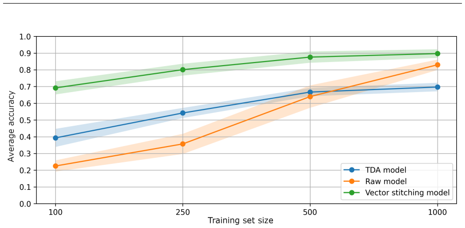
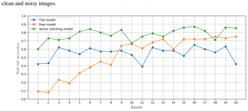
The central discovery is that adding a topological channel to a CNN's input improves classification far beyond what either channel achieves alone. A CNN shown only persistence images reaches about 30% on the hardest protocol; a CNN shown only raw pixels collapses to between 17% and 26%; the stitched model reaches 70-82% on clean-trained sets and 90% when trained on a 90/10 clean/noisy mixture. The topological models also reach high accuracy within the first epochs, suggesting the extra channel accelerates learning rather than merely enlarging the model.

Load-bearing premise

The comparison assumes the three networks are matched closely enough in architecture and training that any accuracy gap comes from the topological information, rather than from the larger stitched input or from the binarization step that filters noise.

Editorial extensions

If this is right

If the central claim holds, hybrid TDA-plus-pixels inputs are a practical way to keep small CNNs accurate on noisy images when labeled data are scarce.
Topological features alone are not enough: the TDA-only model saturates well below the stitched model, so the benefit comes from combining topology with raw pixels rather than replacing them.
The early-epoch advantage suggests topological channels act as a strong prior for low-data training, reducing the number of gradient steps needed to reach a given accuracy.
The authors' own limitation note implies the gain may shrink as networks grow or as datasets carry more information; the method's advantage is most clearly demonstrated in the small-data, high-noise regime.

Reading between the lines

Editorial extensions of the paper, not claims the author makes directly.

The reported gap may partly come from the binarization step removing salt-and-pepper noise before topology is computed; the paper does not isolate that effect from the topological summary itself.
A direct causal test would replace the persistence-image tensor with a random or constant tensor of identical shape in the stitched model; equal accuracy would indicate the advantage is not specifically topological.
If the information-theoretic reading is right, the method should transfer to other low-signal domains, such as medical imaging or time series, where objects are characterized more by shape and connectivity than by texture.
The 17-filtration, 34-layer choice is heuristic, so a natural extension is to ablate the number and type of filtrations and measure accuracy against persistence-image resolution.

Share X Bluesky LinkedIn Reddit HN

Editorial analysis

A structured set of objections, weighed in public.

Desk editor's note, referee report, and a circularity audit.

Desk Editor's Note

read the letter

You should know two things about this one. The empirical result is real in the narrow sense: the reported tables are internally consistent, and the Vector-Stitching model does much better than raw and TDA-only baselines on noisy MNIST with small training sets. But the paper's central claim—that the improvement comes from topological information—is not established. The stress-test note is right: the pipeline in Section 2.1 starts with binarization at a fixed threshold, and the persistence images are built entirely from that binarized image. So the V-S model receives raw noisy pixels plus topological summaries of a thresholded, noise-clipped version of the same pixels. Without a control that stitches raw pixels to binarized pixels (or to any other denoised input), you cannot attribute the gain to persistent homology. Binarization alone could plausibly produce most of the effect.

What is actually new is modest: concatenating raw images with 34 persistence-image channels is a direct application of known TDA vectorization, in the same line as Hofer et al. (2018) which the paper cites. The novelty is the particular configuration and the clean-training/noisy-test evaluation on MNIST. What the paper does well is describe the pipeline concretely, report means, standard deviations, and confidence intervals across 10 runs, and include an honest limitations section—the Data Processing Inequality discussion and the note that gains may shrink with larger networks show the authors are not overselling. The tables are credible.

The soft spots are significant, though. Beyond the binarization confound, the three models are only described as having "as similar a total number of parameters as possible." Architecture, optimizer, training schedule, and input tensor shapes are not given. No random or constant control channels are tested. The evidence is one benchmark, MNIST, with test sets of only 100 images. Noise parameters are not specified. Without code or architecture details, the experiment cannot be reproduced, and the specificity of the claim to topology cannot be checked. The information-theoretic discussion in Section 5 is qualitative and does not supply the missing isolation.

Who is this for? Researchers in the TDA-plus-deep-learning subfield who are looking for low-cost input augmentation ideas. They should read it as a suggestive benchmark observation, not a demonstration of mechanism. I would not cite it in the next year, but I would send it to a serious referee. The confounds are fixable—add binarized-image and random-channel controls, report architectures, release code—and the question is worth answering. Right now the paper is a good working paper, not a finished claim.

Referee Report

4 major / 5 minor

Summary. The paper proposes 'Vector Stitching' (V-S), a method that concatenates raw grayscale MNIST images with persistence images computed by a topological data analysis (TDA) pipeline, and compares three CNNs: a raw-image model, a TDA-only model, and the V-S model. Experiments are run on small clean or 90/10 clean/noisy training sets (100 to 1000 images) with noisy test sets, repeated 10 times. The reported results in Tables 1 and 2 show that V-S substantially outperforms the other two models, and the paper interprets this through an information-theoretic discussion in Section 5.

Significance. If the reported empirical advantage is robust, the paper provides a useful demonstration that TDA-derived features can improve CNN classification in low-data, noisy regimes. The authors report means, standard deviations, and confidence intervals over 10 repetitions, and they include an honest limitations subsection. However, the current evidence is a single dataset with one noise setting, the architectures and hyperparameters are not specified, and no control isolates the topological contribution from the binarization/denoising preprocessing. The significance is therefore promising but not yet established at the level claimed in the abstract and introduction.

major comments (4)

[§2.1 and Table 1] The comparison does not isolate the topological contribution from the binarization step. The persistence images are computed exclusively from the binarized image B defined by the fixed threshold 0.4, so the V-S model receives the raw noisy image together with summaries of a thresholded/denoised image. A binarized-image-only control, or a raw-plus-binarized control, is necessary; without it, the large V-S advantage (e.g., 0.693 vs 0.260 at 100 clean training images in Table 1) could be caused by threshold denoising rather than by persistent homology. Please add such control models and report their accuracies.
[§3.2] The three models are not specified beyond having 'as similar a total number of parameters as possible.' Without layer counts, kernel sizes, padding, optimizers, learning rates, batch sizes, epochs, and any regularization or augmentation, the reader cannot assess capacity matching or reproduce the experiments. The RAW model's accuracy in Table 1 decreases from 0.260 at 100 images to 0.167 at 1000 images, which is suspicious and suggests training instability or unmatched hyperparameters rather than a matched comparison. Please provide complete model definitions and training details for all three networks.
[§3.1 and §4] The experimental evidence is restricted to MNIST under one unspecified noise setting. The paper's general claims that TDA improves neural network performance, and that the information-theoretic interpretation explains this improvement, are not supported beyond this single benchmark. The authors should either substantially restrict the scope of the claims or add at least one additional dataset and a small ablation over noise levels (white-noise variance and salt-and-pepper density are not reported anywhere).
[§5.1 and §5.3] The information-theoretic discussion is not a valid derivation of the empirical gain. The 'conditioning theorem' is invoked as 'adding information cannot hurt model performance,' but conditioning reduces entropy in expectation and does not guarantee that a computed summary improves finite-sample classifier accuracy. Since Section 5.3 acknowledges the Data Processing Inequality, Section 5 should be presented explicitly as qualitative interpretation rather than as an explanation of the V-S advantage.

minor comments (5)

[§1.1] In the definition of an abstract simplicial complex, 'all of its subsets belong to V' should read 'belong to F'; the vertices are V, while the subsets of a simplex are faces in the family F.
[§1.3] The text says that the interval [a, a+1] 'corresponds to a 1-dimensional standard simplex'; this is an elementary interval/cube, not a simplex. Please correct the wording.
[Figure 8 caption] Item 2 in the caption is called a 'Persistence diagram,' but the pipeline in Section 2.1 produces a persistence image after vectorization; the caption should use the correct term.
[§3.1] The noise generation is not reproducible: the text does not specify the white-noise distribution/variance or the salt-and-pepper density, nor how the 10 pseudorandom training/test selections were seeded.
[§2.1] The statement that the pipeline generates a persistence image consisting of 34 layers would be easier to verify if the authors stated how the H0 and H1 channels are ordered and combined for the 17 filtrations.

Circularity Check

0 steps flagged · score 0.0 of 10

No circularity: the accuracy comparison is an independent empirical benchmark, and no prediction reduces to a fitted input or to a self-citation chain.

full rationale

The paper's central claim is an empirical comparison between three CNN input regimes on a noisy MNIST benchmark, with accuracies averaged over 10 independent train/test splits. No parameter is fitted to the test set and then renamed as a prediction; no quantity is defined in terms of another quantity that it is supposed to predict. The V-S input is defined in Section 2.2 as a concatenation of raw pixels and persistence images, and persistence images are a deterministic transform of the same raw image through the Section 2.1 pipeline; but a deterministic feature transformation is a standard input construction, not a circular derivation of the observed accuracy gain. There is also no load-bearing self-citation: the external references that justify the ingredients (Adams et al. for persistence images, Garin and Tauzin for the filtrations, McGuire et al. for the claim that raw-trained networks underuse topology) are independent prior work, and none of the paper's premises is justified solely by the present authors' own prior results. The information-theoretic discussion in Section 5 is qualitative interpretation rather than a derivation, and Section 5.3 explicitly acknowledges the Data Processing Inequality, so the authors do not claim the method manufactures information beyond its input; they also concede the effect may shrink with larger networks. Those limitations weaken causal isolation of topology from the accompanying binarization and from input tensor size, but that is an experimental-control concern, not circularity. No specific circular step can be exhibited, so the honest finding is a score of 0.

Assumptions & free parameters 5 free parameters · 4 assumptions · 0 invented entities

The method has no theoretical derivation; performance rests entirely on an empirical comparison. Key choices, such as the binarization threshold, the number of filtrations, and the persistence image resolution, are unablated and their values are not justified. No new physical or mathematical entity is introduced.

free parameters (5)

Binarization threshold = 0.4
Chosen in Section 2.1 without sensitivity analysis; every persistence image depends on it.
Height filtration directions = 8
Chosen in Section 2.1; each direction contributes H0 and H1 layers, so this choice defines most of the 34 input channels.
Radial filtration centers = 9
Chosen in Section 2.1; similarly defines 18 of the 34 layers.
Persistence image resolution and bandwidth = not stated
Section 1.6 defines an n by n pixel grid, but n and the normal distribution bandwidth are not given in the paper; required to reproduce the pipeline.
Noise levels = not stated
White-noise variance and salt-and-pepper density are mentioned in Section 3.1 but their values are never specified, so the exact benchmark cannot be reconstructed.

assumptions (4)

domain assumption A CNN trained on raw pixel data has limited ability to capture topological properties of images.
Invoked from McGuire et al. [5] in the introduction to motivate the method; if false, the premise that topological information is missing is weakened.
domain assumption Adding relevant information cannot hurt performance because conditioning reduces entropy (the conditioning theorem).
Used in Section 5 and the abstract to explain the results; information-theoretic conditioning does not by itself guarantee higher classifier accuracy.
domain assumption Matching total parameter counts is sufficient to make raw, TDA, and stitched models comparable.
Section 3.2 relies on this to attribute accuracy differences to input content; without matching capacity, the comparison is confounded.
standard math Persistence homology and persistence image definitions are correct as given.
Section 1 recaps standard TDA results; this is background, not the load-bearing part of the empirical claim.

how reviews work

0 comments

Cite this review

Pith. "Pith review of Preserving Information: How does Topological Data Analysis improve Neural Network performance?." pith.science (2026). https://pith.science/paper/SYOYYGBX

@misc{pith2026241118410,
  author       = {Pith},
  title        = {Pith review of: Preserving Information: How does Topological Data Analysis improve Neural Network performance?},
  year         = {2026},
  howpublished = {\url{https://pith.science/paper/SYOYYGBX}},
  note         = {Machine review of arXiv:2411.18410}
}

read the original abstract

Artificial Neural Networks (ANNs) require significant amounts of data and computational resources to achieve high effectiveness in performing the tasks for which they are trained. To reduce resource demands, various techniques, such as Neuron Pruning, are applied. Due to the complex structure of ANNs, interpreting the behavior of hidden layers and the features they recognize in the data is challenging. A lack of comprehensive understanding of which information is utilized during inference can lead to inefficient use of available data, thereby lowering the overall performance of the models. In this paper, we introduce a method for integrating Topological Data Analysis (TDA) with Convolutional Neural Networks (CNN) in the context of image recognition. This method significantly enhances the performance of neural networks by leveraging a broader range of information present in the data, enabling the model to make more informed and accurate predictions. Our approach, further referred to as Vector Stitching, involves combining raw image data with additional topological information derived through TDA methods. This approach enables the neural network to train on an enriched dataset, incorporating topological features that might otherwise remain unexploited or not captured by the network's inherent mechanisms. The results of our experiments highlight the potential of incorporating results of additional data analysis into the network's inference process, resulting in enhanced performance in pattern recognition tasks in digital images, particularly when using limited datasets. This work contributes to the development of methods for integrating TDA with deep learning and explores how concepts from Information Theory can explain the performance of such hybrid methods in practical implementation environments.

Figures

Figures reproduced from arXiv: 2411.18410 by the authors.

**Figure 2.** Construction of Vietoris-Rips and Cech complexes. The ˇ Cech complex (on the left) consists only of ˇ 1-simplices because the closed balls do not have a common intersection. The Vietoris-Rips complex (on the right) contains a 2-simplex because the distance between all points is no greater than α. 1.3 Cubical Complexes Analogously to simplicial complexes, cubical complexes are defined, in which instead of simplices, … view at source ↗

**Figure 3.** Filtration of the Vietoris-Rips complex for a range of radii [PITH_FULL_IMAGE:figures/full_fig_p005_3.png] view at source ↗

Figures from the paper (11 more)

**Figure 4.** Figure 4: Construction of a persistence diagram based on the Vietoris-Rips filtration. [PITH_FULL_IMAGE:figures/full_fig_p006_4.png]

**Figure 5.** Figure 5: The process of creating persistence images. [PITH_FULL_IMAGE:figures/full_fig_p007_5.png]

**Figure 6.** Figure 6: Input data processing pipeline diagram. • Binarization: We convert the input images to a binarized form – each pixel is assigned a value of 1 if its value in the original image exceeds a fixed threshold (we use a threshold of 0.4), otherwise, it is assigned the value o…

**Figure 7.** Figure 7: Image processing through the TDA pipeline. The described pipeline generates a persistence image consisting of 34 layers, where each layer corresponds to a separate persistence image calculated for one of 17 filtrations, successively for H0 and H1. 2.2 Vector Stitching …

**Figure 8.** Figure 8: The method of combining the original image with its corresponding persistence image. 1. Raw image 2. [PITH_FULL_IMAGE:figures/full_fig_p009_8.png]

**Figure 9.** Figure 9: Results of the three models trained on clean training sets with confidence intervals. [PITH_FULL_IMAGE:figures/full_fig_p011_9.png]

**Figure 10.** Figure 10: Results of the three models trained on training sets with a 90/10 split between clean and noisy data, with [PITH_FULL_IMAGE:figures/full_fig_p012_10.png]

**Figure 11.** Figure 11: Accuracy results for one of the iterations, epoch by epoch. The training set consists of a mixture of 100 [PITH_FULL_IMAGE:figures/full_fig_p012_11.png]

**Figure 12.** Figure 12: Accuracy results for one of the iterations, epoch by epoch. The training set consists of a mixture of 250 [PITH_FULL_IMAGE:figures/full_fig_p013_12.png]

**Figure 13.** Figure 13: Accuracy results for one of the iterations, epoch by epoch. The training set consists of a mixture of 500 [PITH_FULL_IMAGE:figures/full_fig_p013_13.png]

**Figure 14.** Figure 14: Accuracy results for one of the iterations, epoch by epoch. The training set consists of a mixture of 1000 [PITH_FULL_IMAGE:figures/full_fig_p013_14.png]

Discussion (0). Continue with ORCID to comment.

Reference graph

Works this paper leans on

27 extracted references · 19 canonical work pages

[1]

Chazal, B

F. Chazal, B. Michel. An Introduction to Topological Data Analysis: Fundamental and Practical Aspects for Data Scientists. Frontiers in Artificial Intelligence, 2021. 15

work page 2021
[2]

Carlsson

G. Carlsson. Topology and Data. Bulletin of The American Mathematical Society - BULL AMER MATH SOC, vol. 46, pp. 255–308, Apr. 2009. DOI: 10.1090/S0273-0979-09-01249-X

doi:10.1090/s0273-0979-09-01249-x 2009
[3]

O’Shea, R

K. O’Shea, R. Nash. An Introduction to Convolutional Neural Networks. ArXiv e-prints, 2015

work page 2015
[4]

Bhanumathi, R

V . Bhanumathi, R. Sangeetha. CNN Based Training and Classification of MRI Brain Images . 2019 5th International Conference on Advanced Computing & Communication Systems (ICACCS), pp. 129–133, 2019. DOI: 10.1109/ICACCS.2019.8728447

work page arXiv 2019
[5]

McGuire, S

S. McGuire, S. Jackson, T. Emerson, H. Kvinge. Do neural networks trained with topological features learn different internal representations? Proceedings of the 1st NeurIPS Workshop on Symmetry and Geometry in Neural Representations, vol. 197, pp. 122–136, Mar. 2023

work page 2023
[6]

Adams, T

H. Adams, T. Emerson, M. Kirby, R. Neville, C. Peterson, P. Shipman, S. Chepushtanova, E. Hanson, F. Motta, L. Ziegelmeier. Persistence Images: A Stable Vector Representation of Persistent Homology. Journal of Machine Learning Research, vol. 18, no. 8, pp. 1–35, 2017

work page 2017
[7]

Bubenik, P

P. Bubenik, P. Dłotko. A persistence landscapes toolbox for topological statistics . Journal of Symbolic Computation, vol. 78, pp. 91–114, 2017. DOI: 10.1016/j.jsc.2016.03.009

doi:10.1016/j.jsc.2016.03.009 2017
[8]

Hofer, R

C. Hofer, R. Kwitt, M. Niethammer, A. Uhl. Deep Learning with Topological Signatures. arXiv:1707.04041, 2018

arXiv 2018

Show all 27 references

[9]

P. O. de Mendez. Geometric Realization of Simplicial Complexes . Graph Drawing. Berlin, Heidelberg: Springer Berlin Heidelberg, pp. 323–332, 1999. ISBN: 978-3-540-46648-2

1999
[10]

de Silva, R

V . de Silva, R. Ghrist. Coordinate-free coverage in sensor networks with controlled boundaries via ho- mology. The International Journal of Robotics Research, vol. 25, no. 12, pp. 1205–1222, 2006. DOI: 10.1177/0278364906072252

2006 doi
[11]

Muhammad, A

A. Muhammad, A. Jadbabaie. Dynamic Coverage Verification in Mobile Sensor Networks Via Switched Higher Order Laplacians. June 2007. DOI: 10.15607/RSS.2007.III.039

2007 doi
[12]

Kaczynski, K

T. Kaczynski, K. Mischaikow, M. Mrozek. Computational Homology. Springer New York, NY , 2004

2004
[13]

Zomorodian, G

A. Zomorodian, G. Carlsson. Computing Persistent Homology. Discrete & Computational Geometry, vol. 33, no. 2, pp. 249–274, Feb. 2005. DOI: 10.1007/s00454-004-1146-y

2005 doi
[14]

E. H. Spanier. The Mayer Homology Theory, 1949

1949
[15]

C. Park, P. Pranav, P. Chingangbam, R. van de Weygaert, B. Jones, G. Vegter, I. Kim, J. Hidding, W. A. Hellwing. Betti numbers of Gaussian fields. Journal of Korean Astronomical Society, vol. 46, July 2013. DOI: 10.5303/JKAS.2013.46.3.125

2013 doi
[16]

Di Fabio, M

B. Di Fabio, M. Ferri. Comparing Persistence Diagrams Through Complex Vectors. Image Analysis and Processing — ICIAP 2015. Cham: Springer International Publishing, pp. 294–305, 2015. ISBN: 978-3-319- 23231-7

2015
[17]

Bubenik.Statistical Topological Data Analysis using Persistence Landscapes

P. Bubenik.Statistical Topological Data Analysis using Persistence Landscapes. Journal of Machine Learning Research, vol. 16, no. 3, pp. 77–102, 2015

2015
[18]

D. Ali, A. Asaad, M. Jimenez, V . Nanda, E. Paluzo-Hidalgo, M. Soriano-Trigueros.A Survey of Vectorization Methods in Topological Data Analysis. IEEE Transactions on Pattern Analysis & Machine Intelligence, vol. 45, no. 12, pp. 14069–14080, Dec. 2023. DOI: 10.1109/TPAMI.2023.3308391

2023
[19]

L. Deng. The mnist database of handwritten digit images for machine learning research . IEEE Signal Processing Magazine, vol. 29, no. 6, pp. 141–142, 2012

2012
[20]

https://github.com/giotto-ai, access date: 07.05.2024

Giotto-AI project. https://github.com/giotto-ai, access date: 07.05.2024. 16

2024
[21]

Tauzin, U

G. Tauzin, U. Lupo, L. Tunstall, J. Burella Pérez, M. Caorsi, A. Medina-Mardones, A. Dassatti, K. Hess. giotto-tda: A Topological Data Analysis Toolkit for Machine Learning and Data Exploration. 2020. arXiv:2004.02551 [cs.CG]

2020 arXiv
[22]

GUDHI User and Reference Manual

The GUDHI Project. GUDHI User and Reference Manual . 3.9.0. GUDHI Editorial Board, 2023. URL: https://gudhi.inria.fr/doc/3.9.0/. access date: 15.06.2024

2023
[23]

Garin, G

A. Garin, G. Tauzin. A Topological "Reading" Lesson: Classification of MNIST using TDA. 2019 18th IEEE International Conference On Machine Learning And Applications (ICMLA), pp. 1551–1556, 2019. DOI: 10.1109/ICMLA.2019.00256

2019
[24]

Singh, C

Y . Singh, C. M. Farrelly, Q. A. Hathaway, et al.Topological Data Analysis in Medical Imaging: Current State of the Art. Insights Imaging, vol. 14, no. 1, p. 58, 2023. DOI: 10.1186/s13244-023-01413-w

2023 doi
[25]

Bresten, J

C. Bresten, J. H. Jung. Detection of Gravitational Waves Using Topological Data Analysis and Convolutional Neural Network: An Improved Approach. arXiv:1910.08245, Oct. 2019

1910 arXiv
[26]

J. A. Thomas, T. M. Cover. Elements of Information Theory. John Wiley Sons, Inc., 2005

2005
[27]

Vaswani, N

A. Vaswani, N. Shazeer, N. Parmar, J. Uszkoreit, L. Jones, A. N. Gomez, Ł. Kaiser, I. Polosukhin.Attention is All You Need. Advances in Neural Information Processing Systems, vol. 30, 2017. 17

2017

Pith tools

Reviewed August 12, 2026 · model on record in the stance chip above.

[1] [1]

Chazal, B

F. Chazal, B. Michel. An Introduction to Topological Data Analysis: Fundamental and Practical Aspects for Data Scientists. Frontiers in Artificial Intelligence, 2021. 15

work page 2021

[2] [2]

Carlsson

G. Carlsson. Topology and Data. Bulletin of The American Mathematical Society - BULL AMER MATH SOC, vol. 46, pp. 255–308, Apr. 2009. DOI: 10.1090/S0273-0979-09-01249-X

doi:10.1090/s0273-0979-09-01249-x 2009

[3] [3]

O’Shea, R

K. O’Shea, R. Nash. An Introduction to Convolutional Neural Networks. ArXiv e-prints, 2015

work page 2015

[4] [4]

Bhanumathi, R

V . Bhanumathi, R. Sangeetha. CNN Based Training and Classification of MRI Brain Images . 2019 5th International Conference on Advanced Computing & Communication Systems (ICACCS), pp. 129–133, 2019. DOI: 10.1109/ICACCS.2019.8728447

work page arXiv 2019

[5] [5]

McGuire, S

S. McGuire, S. Jackson, T. Emerson, H. Kvinge. Do neural networks trained with topological features learn different internal representations? Proceedings of the 1st NeurIPS Workshop on Symmetry and Geometry in Neural Representations, vol. 197, pp. 122–136, Mar. 2023

work page 2023

[6] [6]

Adams, T

H. Adams, T. Emerson, M. Kirby, R. Neville, C. Peterson, P. Shipman, S. Chepushtanova, E. Hanson, F. Motta, L. Ziegelmeier. Persistence Images: A Stable Vector Representation of Persistent Homology. Journal of Machine Learning Research, vol. 18, no. 8, pp. 1–35, 2017

work page 2017

[7] [7]

Bubenik, P

P. Bubenik, P. Dłotko. A persistence landscapes toolbox for topological statistics . Journal of Symbolic Computation, vol. 78, pp. 91–114, 2017. DOI: 10.1016/j.jsc.2016.03.009

doi:10.1016/j.jsc.2016.03.009 2017

[8] [8]

Hofer, R

C. Hofer, R. Kwitt, M. Niethammer, A. Uhl. Deep Learning with Topological Signatures. arXiv:1707.04041, 2018

arXiv 2018