Harnessing Loss Decomposition for Long-Horizon Wave Predictions via Deep Neural Networks

Indu Kant Deo; Rajeev Jaiman

REVIEW 4 major objections 5 minor 22 references

Harnessing Loss Decomposition for Long-Horizon Wave Predictions via Deep Neural Networks

T0 review · 4 major / 5 minor · reviewed 2026-08-11 · deepseek-v4-flash

Challenge this review Re-run · record.json Download PDF Read on arXiv ↗ Review JSON

Pith's one-line read A loss function that tracks phase and amplitude separately keeps neural wave forecasts accurate for longer.

desk verdict A standard MSE decomposition applied to wave forecasting, but the central claim rests on one uncontrolled test case and an inconsistent hyperparameter description. read the letter →

arxiv 2412.02924 v1 pith:7PLVWXE6 submitted 2024-12-04 cs.LG

Indu Kant Deo , Rajeev Jaiman This is my paper · ORCID

classification cs.LG MSC 68T0765M06

keywords lossdecompositionphaseerroramplitudedispersiondissipationlong-horizonpredictionwavepropagationdeepneuralnetworks

verification ladder T0 review T1 audit T2 compute T3 formal

The pith

A machine-rendered reading of the paper's core claim, the machinery that carries it, and where it could break.

The reading

This paper tries to establish that the error accumulation that limits neural network forecasts of wave propagation can be reduced by splitting the training loss into phase and amplitude parts instead of using plain mean squared error. The key identity rewrites MSE as a dissipation term (differences in variance and mean) plus a dispersion term (a correlation deficit), and the authors train their autoencoder with a reweighted combination that emphasizes the propagator and the dispersion error. On a linear advection problem with random wave speeds, the decomposed loss reportedly keeps predictions phase-aligned over the full horizon and lowers error growth relative to an MSE-trained model. If true, this gives a cheap, architecture-independent way to inject numerical concepts of dissipation and dispersion into deep learning for physical forecasting.

What carries the argument

The load-bearing object is a statistical rewriting of MSE into two named error types borrowed from numerical analysis: dissipation (amplitude error) and dispersion (phase error). Concretely, if $u_a$ is the ground truth and $u_d$ the prediction, Eq. 4 reads $$\tau = [\$\sigma$(u_a)-\$\sigma$(u_d)]^2 + (\bar{u}_a - \bar{u}_d)^2 + 2(1-\rho)\$\sigma$(u_a)\$\sigma$(u_d),$$ and the paper defines $\tau_{\mathrm{DISS}}$ as the first two terms and $\tau_{\mathrm{DISP}}$ as the third. The machinery works by giving the optimizer a target that can penalize a wave shape that is right in magnitude but shifted in time differently from a wave that has the right phase but wrong height, which plain MSE cannot distinguish.

What would settle it

Compare the decomposed loss against MSE on two controlled data sets, one where the only error is a time shift (pure phase error, no amplitude change) and one where the only error is amplitude scaling (pure dissipation, no phase shift); if the decomposed loss does not reduce error on the pure phase-shift case, or if it fails to beat MSE on more than the single reported test parameter, the claimed mechanism is not supported.

Watch

Extended reading notes

Core claim

The central claim is that decomposing the mean squared error into separate dissipation and dispersion components, and weighting those components differently during training, substantially improves long-horizon predictions for wave propagation. For the linear advection equation, the authors use the identity $\tau = [\sigma(u_a)-\sigma(u_d)]^2 + (\bar{u}_a - \bar{u}_d)^2 + 2(1-\rho)\sigma(u_a)\sigma(u_d)$, call the first two terms dissipation error and the third term dispersion error, and train the AB-CRAN model with $L_{\mathrm{propagator}} = (1-\beta)\tau_{\mathrm{DISP}} + \beta\tau_{\mathrm{DISS}}$, with hyperparameters favoring the propagator and dispersion. On a held-out wave speed, the model trained this way preserves phase across the prediction horizon, while the MSE-trained model shows phase lag; error-versus-time comparisons show reduced error accumulation. The authors regard this as a framework that can extend to nonlinear wave propagation and other physical forecasting tasks such as fluid dynamics and climate modeling.

Load-bearing premise

The argument depends on the claim that the variance, mean, and correlation statistics in Eq. 5 isolate physical amplitude error from physical phase error; if those statistics mix the two error types, the weighted loss is just arbitrary reweighting of MSE with no guaranteed advantage.

Editorial extensions

If this is right

Networks trained with the decomposed loss should stay phase-aligned over the full rollout, whereas MSE-trained networks develop a growing phase lag.
The usable forecast horizon, meaning the number of time steps before error exceeds a fixed threshold, increases for the linear advection problem.
The improvement transfers to nonlinear wave propagation, since the authors note the approach has been applied to the inviscid Burgers equation.
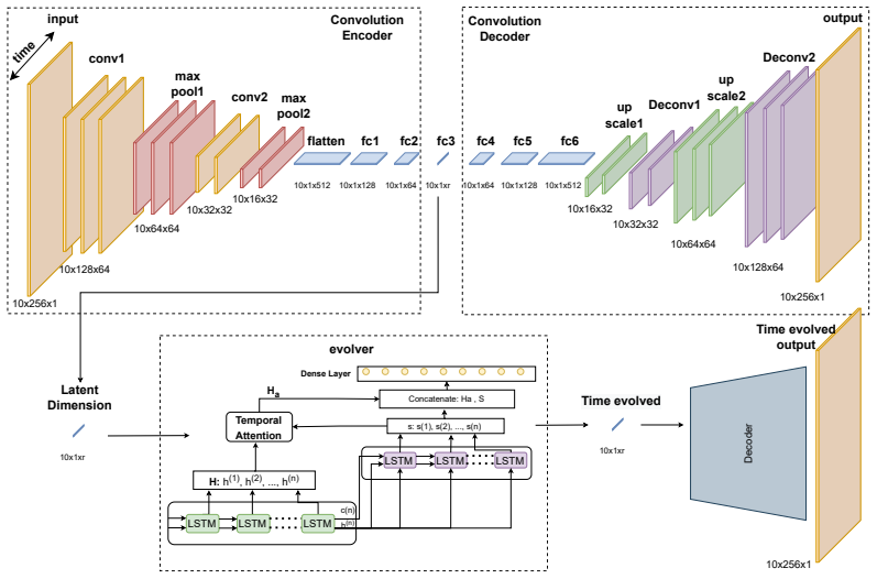
The same weighting strategy, emphasizing the propagator and the dispersion term, can be carried over to other autoregressive spatiotemporal forecasters without changing their architecture.

Reading between the lines

Editorial extensions of the paper, not claims the author makes directly.

Because the dispersion term is a correlation-based statistic, it could serve as a standalone diagnostic for phase drift in any autoregressive model, independent of training.
The behavior of the decomposition at small batch sizes may differ from full-horizon statistics, so its effectiveness could depend on batch size in ways plain MSE does not exhibit.
A testable extension is a training schedule that varies the relative weight of dissipation and dispersion over time, for instance emphasizing amplitude early and phase later, which the paper does not explore.

Share X Bluesky LinkedIn Reddit HN

Signed reviews

No signed human review yet.

Editorial analysis

A structured set of objections, weighed in public.

Desk editor's note, referee report, and a circularity audit.

Desk Editor's Note

read the letter

The loss decomposition in Eqs. 3-5 is the textbook variance-covariance identity for mean squared error. The paper is honest that Le Guen and Thome already applied this idea to time-series forecasting, so the novelty here is limited to the application domain (linear advection) and the AB-CRAN architecture. The algebra is correct, and the authors do report some training details (285 epochs, Ray Tune for alpha and beta). That is the extent of the credit I can give. The empirical claim is the problem. 'Significantly improves phase accuracy' and 'extends the prediction horizon' are supported by one randomly selected test parameter, mu=1.0125, two qualitative figures, and one error-vs-time curve. No aggregate errors across the 19 test instances, no confidence intervals, no ablations, no stated values for alpha and beta. The MSE baseline's hyperparameters and seeds are not reported. Since the loss is a reweighting of an identity, any observed improvement could simply come from tuning alpha and beta on the test case. The single-case comparison cannot carry the generalization claim. There is also an internal inconsistency in the method description. The text says that alpha and beta greater than 0.5 give 'a stronger emphasis on reducing dispersion error,' but Eq. 6 defines Lpropagator = (1-beta)*tau_DISP + beta*tau_DISS. Larger beta puts more weight on tau_DISS, i.e., dissipation, not dispersion. Either the equation or the text is wrong, and without the actual tuned values we cannot tell which was used. This is load-bearing because the whole story is about prioritizing dispersion. A subtler issue: tau_DISP = 2(1-rho)*sigma_a*sigma_d is a Pearson-correlation term, not a pure phase-error metric. It responds to any waveform decorrelation and saturates for large phase shifts. The claim that the decomposition cleanly separates phase and amplitude errors is therefore not established by the math alone. The paper is a workshop note, and that is the level of evidence it provides. The idea is not worthless; there may be a useful empirical study hiding here, but as written the data do not support the conclusions. I would not cite it, and I would not send it to a serious journal as is. My recommendation to the editor: desk reject, with an invitation to resubmit if the authors provide per-test-parameter error statistics, report alpha and beta, fix the inconsistency, and add ablations against plain MSE with matched tuning.

Referee Report

4 major / 5 minor

Summary. The paper proposes to improve long-horizon wave predictions made by an attention-based convolutional recurrent autoencoder by decomposing the mean squared error (MSE) into dissipation and dispersion components. In Section 2.3, the authors rewrite MSE as the sum of a variance-difference term, a mean-difference term, and a correlation term, calling the first two the dissipation error and the third the dispersion error. The training loss then reweights these two error terms (and the decoder versus propagator losses) with hyperparameters α and β. Section 3 evaluates the method on the linear advection equation for one test parameter (μ = 1.0125), with qualitative space-time plots and an error-versus-time curve comparing the decomposed loss against plain MSE. The authors conclude that the proposed loss significantly improves phase accuracy and extends the prediction horizon.

Significance. If the empirical claims were established, the proposed loss decomposition would be a simple and broadly applicable training objective for autoregressive neural network surrogates of wave-like PDEs. The algebraic derivation of the decomposition from MSE is correct and clearly presented, and the paper usefully connects numerical dissipation/dispersion concepts to loss design for deep learning. However, the current evidence is not sufficient for a journal-level claim: the central assertion of phase-accuracy improvement rests on a single test parameter, two qualitative figures, and no reported hyperparameter values. The contribution is therefore more of a promising idea with a proof-of-concept than a validated method.

major comments (4)

[Section 2.3, Eq. (6)] The text states that setting α and β greater than 0.5 puts a stronger emphasis on reducing dispersion error, but in Eq. (6) β multiplies τDISS (the dissipation term), so β > 0.5 actually increases the weight on amplitude error, not phase error. The final tuned values of α and β are not reported anywhere, so the method as described is internally inconsistent and cannot be reproduced or interpreted. Please correct the description and report the actual tuned values, or reconcile the text with the equation.
[Section 3, Figure 4] The paper's central claim that the decomposed loss 'significantly improves phase accuracy' and 'extends the prediction horizon' is supported only by a single randomly selected test parameter (μ = 1.0125), one error-versus-time curve, and no quantitative error metrics, confidence intervals, or results across the other 18 test parameters. A journal-level claim requires aggregate statistics over the full test set, together with a description of the MSE baseline's hyperparameter tuning budget so that the comparison is fair. Without this, the observed improvement could be due to tuning the reweighting coefficients rather than to the decomposition itself.
[Section 2.3, Eq. (5)] The dispersion term τDISP = 2(1 − ρ)σ(ua)σ(ud) is a Pearson-correlation-based measure of overall waveform decorrelation, not a pure phase-error metric: it also responds to amplitude mismatch or any shape change, and it saturates for large phase shifts. The claim that the decomposition cleanly separates phase and amplitude errors is therefore not established. A concrete test would be to evaluate τDISS and τDISP for synthetic perturbations with known pure phase shifts and pure amplitude changes, and to show that they behave as claimed; alternatively, compare against a direct phase-lag metric such as cross-correlation lag.
[Section 2.3 and Section 2.4] The hyperparameters α and β are tuned using Ray Tune ASHA, but the search ranges, the number of trials, and the final selected values are not reported. Because Eq. (4) is an algebraic identity, any choice of α and β is just a reweighted MSE; the paper's claim of a principled advantage requires demonstrating that the selected weights are robust across the test set and that plain MSE trained with the same tuning effort does not match the performance. Please provide these details.

minor comments (5)

[Abstract and Section 2.3] The phrase 'novel theoretical framework' overstates what Eq. (4) provides, since the decomposition is an algebraic identity; consider rephrasing to 'loss reweighting strategy' or 'decomposition-based loss formulation'.
[Section 2.4] The denoising decoder loss is mentioned but no ablation or description of its interaction with the decomposed propagator loss is given; clarify whether the reported improvement is attributed to the decomposition alone or to the combination with denoising.
[Figure 4 caption] The caption says 'with a time-horizon of 10 time-steps', while the paper discusses long-horizon predictions; please clarify the relationship between this horizon, the 200 simulated time steps, and the non-dimensional times t* = 0.036 and 0.392.
[Section 3] The phrase 'We randomly selected a parameter from the test set' is vague; specify the selection procedure and, ideally, report results for all 19 test parameters rather than only one.
[Throughout] There are several presentation issues: the typo 'Coodinate' in Figure 3, the inconsistent use of 'AB-CRAN' before it is defined, and some incomplete reference formatting (e.g., [15]). These should be corrected.

Circularity Check

1 steps flagged · score 4.0 of 10

Loss decomposition is an algebraic identity relabeled as phase/amplitude errors; the empirical comparison is independent but weakly controlled.

self definitional [Section 2.3, Eqs. (4)-(6); Section 3, Figure 4 and accompanying text]
"We define the first two terms of the RHS of Eq. 4 as the dissipation error and the third term as the dispersion error: τDISS = [σ (ua) − σ (ud)]2 + (¯ua − ¯ud)2 , τDISP = 2(1 − ρ)σ (ua) σ (ud) . (5) We employ this decomposition to formulate the loss function as follows: Lfunction = (1 − α)LDecoder + αLpropagator , Lpropagator = (1 − β)τDISP + βτDISS , (6)"

The two 'error components' in Eq. (5) are not derived from numerical analysis; they are simply the two groups of terms in the algebraic identity Eq. (4), for which τDISS + τDISP equals the MSE exactly. The loss in Eq. (6) is therefore a reweighted combination of the two parts of that identity, so the decomposition carries no independent information beyond the MSE statistics. The paper then attributes the empirical improvement to 'separately addressing phase and amplitude errors,' but 'phase error' is only a name given to τDISP; no independent phase-error metric establishes that τDISP isolates phase lag.

full rationale

The paper's derivation chain contains no formal circularity in the sense of fitting a parameter and then predicting that same parameter; Eq. (4) is a correct identity for MSE, and Eq. (5) is a definitional naming of its terms. The claimed improvement in phase accuracy is an empirical comparison between models trained with MSE and with the reweighted loss, and that comparison is not forced by the identity, so the central empirical claim has independent content. However, the paper's interpretive step is circular: 'dispersion error' is defined as τDISP, and the success is then attributed to reducing phase error without independently validating that τDISP measures phase. The tuned weights α and β are fit on data, and the statement that β>0.5 'emphasizes dispersion' is inconsistent with Eq. (6), where β multiplies τDISS; these issues weaken the explanation but are largely correctness risks rather than circularity. The architecture is taken from the authors' prior self-citation, but the loss-decomposition claim does not rest on that citation. Overall, the empirical result is not a derived prediction and the decomposition is not load-bearing support for the numerical comparison; the score reflects the definitional relabeling rather than full circularity.

Assumptions & free parameters 2 free parameters · 3 assumptions · 0 invented entities

The method introduces no new physical entities. The free parameters are the loss weights alpha and beta, tuned on data and not reported. The central assumptions are the algebraic identity, the physical interpretation of the decomposition, and the transferability of the fixed architecture.

free parameters (2)

alpha (α) = not reported, tuned via Ray Tune ASHA, greater than 0.5
Weight balancing decoder loss and propagator loss; tuned on data, not derived.
beta (β) = not reported, tuned via Ray Tune ASHA, greater than 0.5 with emphasis on dispersion
Weight balancing dispersion and dissipation error terms; tuned on data; the reported improvement is contingent on this choice.

assumptions (3)

standard math The variance/covariance decomposition of mean squared error in Eqs. 3-5 is a valid algebraic identity.
The decomposition follows from the definition of variance and covariance; the paper uses it as the theoretical basis.
domain assumption The dissipation and dispersion terms in Eq. 5 correspond to amplitude and phase errors in wave propagation.
The paper asserts this correspondence without derivation; for phase-shifted fields, variance and mean terms can also change, so the mapping is not exact.
domain assumption The AB-CRAN architecture and its hyperparameters from Deo et al. [5] are fixed and appropriate for this problem.
The method is only tested with this architecture and these settings, so claims of general applicability assume they transfer.

how reviews work

0 comments

Cite this review

Pith. "Pith review of Harnessing Loss Decomposition for Long-Horizon Wave Predictions via Deep Neural Networks." pith.science (2026). https://pith.science/paper/7PLVWXE6

@misc{pith2026241202924,
  author       = {Pith},
  title        = {Pith review of: Harnessing Loss Decomposition for Long-Horizon Wave Predictions via Deep Neural Networks},
  year         = {2026},
  howpublished = {\url{https://pith.science/paper/7PLVWXE6}},
  note         = {Machine review of arXiv:2412.02924}
}

read the original abstract

Accurate prediction over long time horizons is crucial for modeling complex physical processes such as wave propagation. Although deep neural networks show promise for real-time forecasting, they often struggle with accumulating phase and amplitude errors as predictions extend over a long period. To address this issue, we propose a novel loss decomposition strategy that breaks down the loss into separate phase and amplitude components. This technique improves the long-term prediction accuracy of neural networks in wave propagation tasks by explicitly accounting for numerical errors, improving stability, and reducing error accumulation over extended forecasts.

Figures

Figures reproduced from arXiv: 2412.02924 by the authors.

**Figure 2.** Illustration of attention-based convolutional recurrent autoencoder architecture. [PITH_FULL_IMAGE:figures/full_fig_p003_2.png] view at source ↗

**Figure 3.** Linear convection problem: Exact solution (left), AB-CRAN solution with n = 2 (center) [PITH_FULL_IMAGE:figures/full_fig_p004_3.png] view at source ↗

Figures from the paper (1 more)

**Figure 4.** Figure 4: Accuracy assessment for wave prediction: (a) Comparison of MSE-based loss and Loss [PITH_FULL_IMAGE:figures/full_fig_p005_4.png]

Discussion (0). Continue with ORCID to comment.

Reference graph

Works this paper leans on

22 extracted references · 16 canonical work pages

[1]

Abadi et al

M. Abadi et al. TensorFlow: Large-scale machine learning on heterogeneous systems, 2015. URL https://www.tensorflow.org/. Software available from tensorflow.org

work page 2015
[2]

Computational fluid dynamics, volume 206

John David Anderson and John Wendt. Computational fluid dynamics, volume 206. Springer, 1995. 5

work page 1995
[3]

Zico Kolter, and Vladlen Koltun

Shaojie Bai, J. Zico Kolter, and Vladlen Koltun. An empirical evaluation of generic convo- lutional and recurrent networks for sequence modeling. arXiv preprint arXiv:1803.01271 , 2018

arXiv 2018
[4]

Enforcing analytic constraints in neural networks emulating physical systems

Tom Beucler, Michael Pritchard, Stephan Rasp, Jordan Ott, Pierre Baldi, and Pierre Gentine. Enforcing analytic constraints in neural networks emulating physical systems. Physical Review Letters, 126(9):098302, 2021

work page 2021
[5]

Predicting waves in fluids with deep neural network.Physics of Fluids, 34(6), 2022

Indu Kant Deo and Rajeev Jaiman. Predicting waves in fluids with deep neural network.Physics of Fluids, 34(6), 2022

work page 2022
[6]

Combined space–time reduced-order model with three-dimensional deep convolution for extrapolating fluid dynamics

Indu Kant Deo, Rui Gao, and Rajeev Jaiman. Combined space–time reduced-order model with three-dimensional deep convolution for extrapolating fluid dynamics. Physics of Fluids, 35(4), 2023

work page 2023
[7]

Predicting wave propagation for varying bathymetry using conditional convolutional autoencoder network

Indu Kant Deo, Akash Vankateshwaran, and Rajeev Jaiman. Predicting wave propagation for varying bathymetry using conditional convolutional autoencoder network. In International Conference on Offshore Mechanics and Arctic Engineering, volume 87844, page V006T08A038. American Society of Mechanical Engineers, 2024

work page 2024
[8]

Continual Learning of Range-Dependent Transmission Loss for Underwater Acoustic using Conditional Convolutional Neural Net

Indu Kant Deo, Akash Venkateshwaran, and Rajeev K Jaiman. Continual learning of range- dependent transmission loss for underwater acoustic using conditional convolutional neural net. arXiv preprint arXiv:2404.08091, 2024

work page Pith review arXiv 2024

Show all 22 references

[9]

A finite element-inspired hypergraph neural network: Application to fluid dynamics simulations

Rui Gao, Indu Kant Deo, and Rajeev K Jaiman. A finite element-inspired hypergraph neural network: Application to fluid dynamics simulations. Journal of Computational Physics, 504: 112866, 2024

2024
[10]

Deep convolutional recurrent autoencoders for learning low-dimensional feature dynamics of fluid systems

Francisco J Gonzalez and Maciej Balajewicz. Deep convolutional recurrent autoencoders for learning low-dimensional feature dynamics of fluid systems. arXiv preprint arXiv:1808.01346, 2018

2018 arXiv
[11]

Deep Learning

Ian Goodfellow, Yoshua Bengio, and Aaron Courville. Deep Learning. MIT Press, 2016. URL http://www.deeplearningbook.org

2016
[12]

Griffiths

Graham W. Griffiths. Dissipation and Dispersion, page 264–284. Cambridge University Press, 2016

2016
[13]

Theory-guided data science: A new paradigm for scientific discovery from data

Anuj Karpatne, Gowtham Atluri, James H Faghmous, Michael Steinbach, Arindam Banerjee, Auroop Ganguly, Shashi Shekhar, Nagiza Samatova, and Vipin Kumar. Theory-guided data science: A new paradigm for scientific discovery from data. IEEE Transactions on knowledge and data engine...

2017
[14]

Comparison of accurate methods for the integration of hyperbolic equations

Heinz-Otto Kreiss and Joseph Oliger. Comparison of accurate methods for the integration of hyperbolic equations. Tellus, 24:199–215, 1972. doi: 10.1111/j.2153-3490.1972.tb01584.x

1972
[15]

Shape and time distortion loss for training deep time series forecasting models

Vincent Le Guen and Nicolas Thome. Shape and time distortion loss for training deep time series forecasting models. Advances in neural information processing systems, 32, 2019

2019
[16]

Deep learning

Yann LeCun, Yoshua Bengio, and Geoffrey Hinton. Deep learning. Nature, 521:436–444, 2015. doi: 10.1038/nature14539

2015 doi
[17]

R. J. LeVeque et al. Finite volume methods for hyperbolic problems, volume 31. Cambridge university press, 2002

2002
[18]

A system for massively parallel hyperparameter tuning

Liam Li, Kevin Jamieson, Afshin Rostamizadeh, Ekaterina Gonina, Jonathan Ben-Tzur, Moritz Hardt, Benjamin Recht, and Ameet Talwalkar. A system for massively parallel hyperparameter tuning. Proceedings of Machine Learning and Systems, 2:230–246, 2020

2020
[19]

Sgdr: Stochastic gradient descent with warm restarts

Ilya Loshchilov and Frank Hutter. Sgdr: Stochastic gradient descent with warm restarts. arXiv preprint arXiv:1608.03983, 2016

2016 arXiv
[20]

Prediction error meta classification in semantic segmentation: Detection via aggregated dispersion mea- sures of softmax probabilities

Matthias Rottmann, Lukas Pape, Mark Petersen, Hans Ulmer, and Hanno Gottschalk. Prediction error meta classification in semantic segmentation: Detection via aggregated dispersion mea- sures of softmax probabilities. In IEEE International Conference on Intelligent Transportatio...

2018
[21]

Reduced-order modeling for parameterized pdes via implicit neural representations

Tianshu Wen, Kookjin Lee, and Youngsoo Choi. Reduced-order modeling for parameterized pdes via implicit neural representations. arXiv preprint arXiv:2311.16410, 2023

2023 arXiv
[22]

Understanding adamw through proximal methods and scale-freeness

Zhenxun Zhuang, Mingrui Liu, Ashok Cutkosky, and Francesco Orabona. Understanding adamw through proximal methods and scale-freeness. Transactions on machine learning research, 2022. 6

2022

Pith tools

Reviewed August 11, 2026 · model on record in the stance chip above.

[1] [1]

Abadi et al

M. Abadi et al. TensorFlow: Large-scale machine learning on heterogeneous systems, 2015. URL https://www.tensorflow.org/. Software available from tensorflow.org

work page 2015

[2] [2]

Computational fluid dynamics, volume 206

John David Anderson and John Wendt. Computational fluid dynamics, volume 206. Springer, 1995. 5

work page 1995

[3] [3]

Zico Kolter, and Vladlen Koltun

Shaojie Bai, J. Zico Kolter, and Vladlen Koltun. An empirical evaluation of generic convo- lutional and recurrent networks for sequence modeling. arXiv preprint arXiv:1803.01271 , 2018

arXiv 2018

[4] [4]

Enforcing analytic constraints in neural networks emulating physical systems

Tom Beucler, Michael Pritchard, Stephan Rasp, Jordan Ott, Pierre Baldi, and Pierre Gentine. Enforcing analytic constraints in neural networks emulating physical systems. Physical Review Letters, 126(9):098302, 2021

work page 2021

[5] [5]

Predicting waves in fluids with deep neural network.Physics of Fluids, 34(6), 2022

Indu Kant Deo and Rajeev Jaiman. Predicting waves in fluids with deep neural network.Physics of Fluids, 34(6), 2022

work page 2022

[6] [6]

Combined space–time reduced-order model with three-dimensional deep convolution for extrapolating fluid dynamics

Indu Kant Deo, Rui Gao, and Rajeev Jaiman. Combined space–time reduced-order model with three-dimensional deep convolution for extrapolating fluid dynamics. Physics of Fluids, 35(4), 2023

work page 2023

[7] [7]

Predicting wave propagation for varying bathymetry using conditional convolutional autoencoder network

Indu Kant Deo, Akash Vankateshwaran, and Rajeev Jaiman. Predicting wave propagation for varying bathymetry using conditional convolutional autoencoder network. In International Conference on Offshore Mechanics and Arctic Engineering, volume 87844, page V006T08A038. American Society of Mechanical Engineers, 2024

work page 2024

[8] [8]

Continual Learning of Range-Dependent Transmission Loss for Underwater Acoustic using Conditional Convolutional Neural Net

Indu Kant Deo, Akash Venkateshwaran, and Rajeev K Jaiman. Continual learning of range- dependent transmission loss for underwater acoustic using conditional convolutional neural net. arXiv preprint arXiv:2404.08091, 2024

work page Pith review arXiv 2024