REVIEW 4 major objections 6 minor 34 references
Epidemiological Model Calibration via Graybox Bayesian Optimization
T0 review · 4 major / 6 minor · reviewed 2026-08-11 · deepseek-v4-flash
Pith's one-line read By treating the SIQR compartmental structure as a known function network rather than a black box, graybox Bayesian optimization calibrates epidemic models with fewer simulator evaluations and lower log-MSE than standard BO.
desk verdict Empirically useful graybox BO for SIQR calibration, but the appendix convergence proof has a max/sum interchange error that invalidates Theorem 1 as stated. read the letter →
The pith
A machine-rendered reading of the paper's core claim, the machinery that carries it, and where it could break.
The reading
What carries the argument
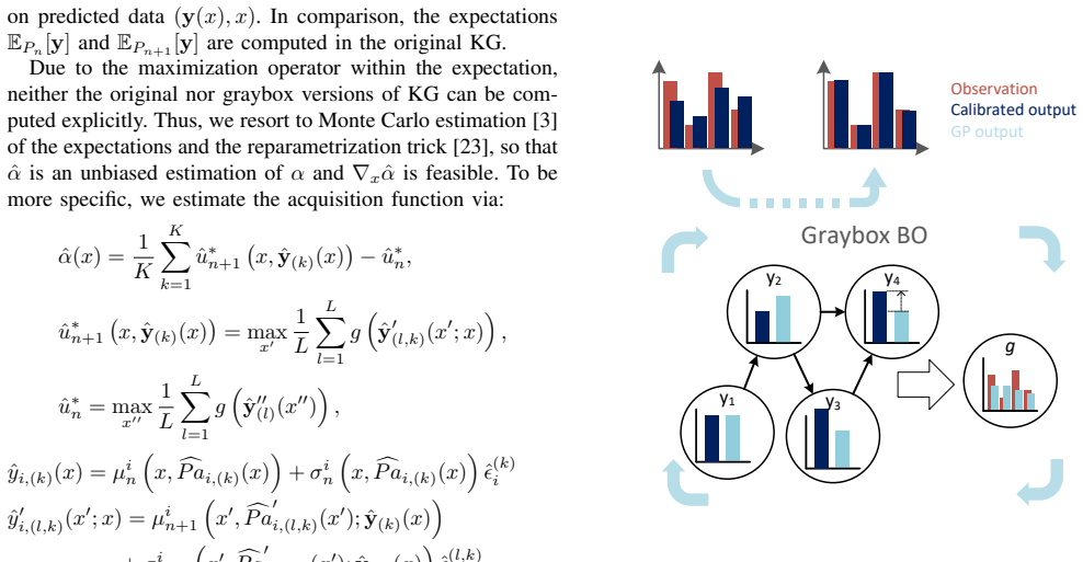
The carrying object is the function network $G(V, E)$ combined with a composite-function objective. $V$ contains the parameter node $x$, four GP nodes $y_1,\dots,y_4$ for S, I, Q, and R, and the metric node $g$; each edge encodes a known dependency, such as I coming from S and R coming from I and Q. The GPs have posterior means and variances conditioned on all previously queried simulator trajectories, and $g(y(x))$ is the known negative MSE, so only the compartment outputs need to be learned. The graybox knowledge-gradient acquisition $\alpha_n(x, z) = \frac{1}{\mathbf{1}^\top z}\mathbb{E}_{P_n(y(x))}[u^*_{n+1}(z, y(x))] - u^*_n$ estimates, for each candidate $x$ and conditioning subset $z$, the expected gain in best achievable metric after one more query; it is evaluated by Monte Carlo with $K=8$ samples, $L=128$ inner samples, and the reparametrization trick, giving unbiased estimates and tractable gradients.
What would settle it
Run the graybox BO procedure on a simulator whose compartment outputs are provably not in the Gaussian process prior's sample paths (for example, a trajectory with a sharp discontinuity induced by a parameter threshold), and check whether $\alpha_n$ still converges to zero and whether the log-MSE still improves at the claimed rate; if the algorithm stalls while black-box BO continues to improve, Assumption 1 is the load-bearing premise.
Extended reading notes
Core claim
The central claim is that integrating structural knowledge of the compartmental model into the BO acquisition loop improves both final calibration error and convergence speed. Instead of one GP on the scalar objective $f(x)$, the paper places separate GPs on the four SIQR compartment trajectories $y_i(x)$, defines the calibration metric $g(y(x))$ as the known negative mean squared error, and organizes the GPs into a function network whose edges encode which compartments feed which. The acquisition function is then a knowledge-gradient expected improvement computed over these GPs, and its decoupled variant chooses a binary vector $z$ indicating which GPs should be conditioned on predicted data before the next simulator query. Experiments over linear, noisy, and nonlinear ground-truth SIQR models, with and without the susceptible compartment observed, show the graybox methods (KG-CF, KG-FN, DG-CF) dominate black-box EI and KG in log-MSE and iteration budget; on U.S. and U.K. COVID-19 infectious-count data, the function-network variant achieves the lowest mean squared error among the compared methods.
Load-bearing premise
The convergence guarantee assumes the true SIQR simulator outputs are functions the Gaussian process prior can represent, and the paper never verifies this for the parameter ranges it calibrates.
Editorial extensions
If this is right
- Calibrating an ODE-based epidemic model requires only tens of simulator evaluations, because the surrogate GPs and the known metric absorb most of the objective's complexity.
- Missing compartments do not destroy calibration: the function network propagates information from observed compartments to the unobserved one.
- The decoupled acquisition lets the optimizer spend its simulation budget on the compartments whose GP surrogates are least reliable, rather than refreshing all four evenly.
- The same graybox recipe transfers to other compartmental variants and to agent-based models whose input-output dependencies can be written as a known graph.
Reading between the lines
- The composite-function/function-network machinery is essentially generic: any expensive simulator with a known scalar summary metric can be calibrated this way, with the SIQR model being one tested instance.
- The decoupled acquisition suggests a natural adaptive-budget rule: allocate simulator queries to compartments with high posterior variance; the paper's $z$ vector provides the per-compartment information such a rule would need, but the paper does not itself propose that rule.
- Because the convergence theorem depends on the GP prior containing the true trajectory, extending the method to highly irregular agent-based model outputs may require nonstationary or warped GP priors, a modification the paper leaves untested.
- A stronger real-data test would use multi-compartment observations rather than infectious counts alone, to see whether the function-network advantage over the composite-function-only variant persists when every compartment is observed noisily.
Editorial analysis
A structured set of objections, weighed in public.
Referee Report
Summary. The paper proposes graybox Bayesian optimization (BO) methods for calibrating compartmental epidemiological SIQR models. It models each compartment output with a Gaussian process, uses the known composite structure of the negative mean-squared-error objective, and introduces a decoupled acquisition function that conditions on predicted outputs from a subset of the GPs. The authors report improved calibration performance, measured by log-MSE, relative to blackbox EI and KG baselines on simulated data, and apply the methods to calibrate SIQR and neural-ODE variants on U.S. and U.K. COVID-19 datasets. An appendix states a convergence theorem for the decoupled acquisition function.
Significance. If the empirical findings hold, the paper presents a practically useful recipe for sample-efficient calibration of expensive epidemiological models, with code provided. The simulated experiments cover complete and incomplete observations, noise, and a nonlinear ground-truth model, and consistently show that the graybox variants outperform blackbox EI and KG within 50 BO iterations. These strengths make the empirical contribution potentially valuable. However, the theoretical convergence claim in the appendix is unsupported due to a mathematically invalid decomposition, and some real-data claims are contradicted by the paper's own table. The conceptual contribution of the function-network graph also needs clarification because the graph as drawn does not encode the SIQR compartment dependencies the text appeals to.
major comments (4)
- [Appendix, proof of Theorem 1] The proof of Theorem 1 assumes that the maximum over x' of a sum of per-compartment expected utilities equals the sum of per-component maxima. Specifically, Eq. (9) defines u^*_{n+1}(z, y(x)) = max_{x'} E_{P_{n+1}(y'(x'); z, y(x))}[g(y')] with g(y') additive over the four compartments, but the proof's final line replaces this with Σ_i z_i G_i^n(x), where each G_i^n uses its own per-component maximizer x'_*. The interchange max_{x'} Σ_i f_i(x') = Σ_i max_{x'} f_i(x') is false in general. Consequently, the bound 0 ≤ α_n(x_n) ≤ Σ_i G_i^n(x_n) is not established, and the claimed convergence α_n → 0 a.s. does not follow. This is a load-bearing error in the paper's theoretical justification; the authors should either provide a correct proof with a common maximizer argument or remove the theorem and clearly state that convergence is not proved.
- [Appendix, Assumption 1] Assumption 1 states that the true computer model η is in the state space of the GP prior y ∼ P_n for n ≥ 1, which is needed for Lemma 2 and hence for Theorem 1. The paper gives no argument that SIQR trajectories over the parameter ranges considered lie in the sample path space or RKHS of a Matérn GP, and the term 'state space' is not defined. This assumption is not merely technical; it is a function-class condition that the ODE solutions may fail. At minimum, the assumption should be stated precisely and its plausibility for the SIQR model should be discussed.
- [Section III.A, Fig. 2, Eq. (5)] The function-network graph in Fig. 2 contains edges only from x to each y_i and from each y_i to g; there are no edges between compartments. According to Eq. (5), P ai = {y_j : (y_j → y_i) ∈ E}, so every P ai is empty, making the KG-FN model identical to KG-CF under the stated graph. The paper nonetheless reports performance differences between KG-FN and KG-CF and attributes them to the 'ground-truth functional dependency' of the SIQR model. This is internally inconsistent: either the implementation uses additional edges that are not shown (such as S→I or I→Q), or the reported differences arise from another source. Please clarify the actual graph used in the experiments and how it relates to the SIQR ODE structure.
- [Section V, Table I] Table I contradicts the sentence claiming that KG-FN is 'generally better with lower variance.' In the U.K. column, KG-FN has mean smallest-MSE 45.0617×10^4 versus 44.6875×10^4 for KG-CF, so KG-FN is worse on average on that dataset. Also, the real-data experiments compare only KG-CF and KG-FN; no blackbox EI or KG baseline is included. Therefore these experiments do not support the abstract's broad claim that graybox variants outperform blackbox BO on real data. The authors should add blackbox baselines to the real-data study or restrict that claim to the simulated experiments.
minor comments (6)
- [Eq. (4) vs. Eq. (3)] The sign of g is inconsistent: Eq. (3) defines g as the negative squared error, while Eq. (4) writes g(y(x)) = (1/T) Σ_i (d_i - y_i(x))^2 without the minus sign. Please align the notation throughout.
- [Throughout] There are several typos, including 'the the commonly adopted' in the Introduction, 'Recoverd' and 'Qurantined' in Figs. 4 and 7, and 'derivation function' in Section IV. A careful proofreading pass is needed.
- [References] Reference [1] lists 'Publisher Full Text' instead of a journal or venue name; this citation is incomplete.
- [Section III.B] The notation g ⊥ v is not defined in the text; please define statistical independence or replace it with a more standard notation such as g ⊥ v meaning 'g is independent of v'.
- [Algorithm 1] Algorithm 1 writes Pn(yi(x)) ← N(µ_i^n(x), σ_i^n(x)), which omits the parent variables P ai used in Eq. (5) and in the acquisition function; this makes the pseudo-code inconsistent with the method description.
- [Section V] The parameter ranges '10^−1 bI(0) ≤ x5 ≤ 10bI(0)' and '10bI(0) ≤ x6 ≤ 10^3 bI(0)' should use explicit multiplication (e.g., 10^{-1} · bI(0)) to avoid ambiguity.
Circularity Check
No circularity found: the paper's central claims are empirical comparisons on simulated and real data, and the convergence theorem is conditional on an explicit assumption rather than defined in terms of its own conclusion.
full rationale
The paper's methods (KG-CF, KG-FN, DG-CF) are introduced as modifications of composite-function/function-network BO from Astudillo and Frazier ([5], [6]), which are not authored by the present paper's researchers, so no self-citation chain carries the argument. The central claim that graybox BO variants calibrate SIQR models more efficiently is supported by experiments on synthetic ground-truth trajectories with known parameters and on real COVID-19 data; reported MSE is computed from the actual SIQR model output after calibration, not from the fitted surrogate, so no fitted quantity is renamed as a prediction. The graybox assumption that g is known and cheap is an architectural choice, not a result derived from the data, so it is not circular. Appendix Theorem 1's convergence statement explicitly assumes eta lies in the GP state space (Assumption 1); stating an assumption is not equivalent to assuming the conclusion. The only potentially load-bearing derivation issue is in the appendix's treatment of the decoupled acquisition as a sum of per-component maxima, but that would be a mathematical correctness gap, not a definitional or fitted-input circularity. Per the review rules, correctness concerns are scored separately from circularity. No circular step can be exhibited with a quotation showing an equation reducing to its own inputs, so the appropriate finding is no significant circularity.
Assumptions & free parameters
free parameters (3)
- Monte Carlo sample sizes K and L =
K=8, L=128
- GP kernel hyperparameters =
MLE estimates per GP
- Initial design size =
2D+1 random points in [0,1]^D
assumptions (4)
- domain assumption Observed data follow d_t = η_t(x) + ε with ε ~ N(0, Diag(1)) (Eq. 2)
- domain assumption η is in the state space of the GP prior (Assumption 1)
- ad hoc to paper The function network graph with edges x to y_i and y_i to g, with no edges between compartments (Fig. 2), captures the structure of the SIQR model
- domain assumption The inner maximizer x' in u^*_{n+1} can be optimized with Monte Carlo estimates using K=8 and L=128 samples (Eq. 7)
Cite this review
Pith. "Pith review of Epidemiological Model Calibration via Graybox Bayesian Optimization." pith.science (2026). https://pith.science/paper/5JMJIPBT
@misc{pith2026241207193,
  author       = {Pith},
  title        = {Pith review of: Epidemiological Model Calibration via Graybox Bayesian Optimization},
  year         = {2026},
  howpublished = {\url{https://pith.science/paper/5JMJIPBT}},
  note         = {Machine review of arXiv:2412.07193}
}
read the original abstract
In this study, we focus on developing efficient calibration methods via Bayesian decision-making for the family of compartmental epidemiological models. The existing calibration methods usually assume that the compartmental model is cheap in terms of its output and gradient evaluation, which may not hold in practice when extending them to more general settings. Therefore, we introduce model calibration methods based on a "graybox" Bayesian optimization (BO) scheme, more efficient calibration for general epidemiological models. This approach uses Gaussian processes as a surrogate to the expensive model, and leverages the functional structure of the compartmental model to enhance calibration performance. Additionally, we develop model calibration methods via a decoupled decision-making strategy for BO, which further exploits the decomposable nature of the functional structure. The calibration efficiencies of the multiple proposed schemes are evaluated based on various data generated by a compartmental model mimicking real-world epidemic processes, and real-world COVID-19 datasets. Experimental results demonstrate that our proposed graybox variants of BO schemes can efficiently calibrate computationally expensive models and further improve the calibration performance measured by the logarithm of mean square errors and achieve faster performance convergence in terms of BO iterations. We anticipate that the proposed calibration methods can be extended to enable fast calibration of more complex epidemiological models, such as the agent-based models.
Figures


Figures from the paper (5 more)


Reference graph
Works this paper leans on
-
[1]
Alberto Aleta, David Martin-Corral, A Piontti, Marco Ajelli, Maria Litvinova, Matteo Chinazzi, et al. Modeling the impact of social distancing, testing, contact tracing and household quarantine on second- wave scenarios of the COVID-19 pandemic. Publisher Full Text, 2021
work page 2021
-
[2]
Data-based analysis, modelling and forecasting of the COVID-19 outbreak
Cleo Anastassopoulou, Lucia Russo, Athanasios Tsakris, and Constanti- nos Siettos. Data-based analysis, modelling and forecasting of the COVID-19 outbreak. PloS one, 15(3):e0230405, 2020
work page 2020
-
[3]
An introduction to MCMC for machine learning
Christophe Andrieu, Nando De Freitas, Arnaud Doucet, and Michael I Jordan. An introduction to MCMC for machine learning. Machine learning, 50:5–43, 2003
work page 2003
-
[4]
Accurate calibration of agent-based epidemiological models with neural network surrogates
Rushil Anirudh, Jayaraman J Thiagarajan, Peer-Timo Bremer, Timothy Germann, Sara Del Valle, and Frederick Streitz. Accurate calibration of agent-based epidemiological models with neural network surrogates. In Workshop on Healthcare AI and COVID-19, pages 54–62. PMLR, 2022
work page 2022
-
[5]
Bayesian optimization of composite functions
Raul Astudillo and Peter Frazier. Bayesian optimization of composite functions. In International Conference on Machine Learning , pages 354–363. PMLR, 2019
work page 2019
-
[6]
Bayesian optimization of function net- works
Raul Astudillo and Peter Frazier. Bayesian optimization of function net- works. Advances in neural information processing systems , 34:14463– 14475, 2021
work page 2021
-
[7]
BOTorch: A framework for efficient Monte-Carlo Bayesian optimization
Maximilian Balandat, Brian Karrer, Daniel Jiang, Samuel Daulton, Ben Letham, Andrew G Wilson, and Eytan Bakshy. BOTorch: A framework for efficient Monte-Carlo Bayesian optimization. Advances in neural information processing systems , 33:21524–21538, 2020
work page 2020
-
[8]
A super- martingale approach to Gaussian process based sequential design of experiments
Julien Bect, Franc ¸ois Bachoc, and David Ginsbourger. A super- martingale approach to Gaussian process based sequential design of experiments. 2019
work page 2019
Show all 34 references
-
[9]
Pa- rameter estimation and prediction for coronavirus disease outbreak 2019 (COVID-19) in Algeria
Soufiane Bentout, Abdennasser Chekroun, and Toshikazu Kuniya. Pa- rameter estimation and prediction for coronavirus disease outbreak 2019 (COVID-19) in Algeria. AIMS Public Health , 7(2):306, 2020
2019
-
[10]
Adaptive recovery model: Designing systems for testing tracing and vaccination to support COVID-19 recovery planning
Walter E Beyeler, Erin Acquesta, Katherine A Klise, Monear Makvandi, and Patrick D Finley. Adaptive recovery model: Designing systems for testing tracing and vaccination to support COVID-19 recovery planning. Technical report, Sandia National Lab.(SNL-NM), Albuquerque, NM (Uni...
2020
-
[11]
Mathematical models in epidemiology , volume 32
Fred Brauer, Carlos Castillo-Chavez, Zhilan Feng, et al. Mathematical models in epidemiology , volume 32. Springer, 2019
2019
-
[12]
Nonparametric functional calibration of computer models
D Andrew Brown and Sez Atamturktur. Nonparametric functional calibration of computer models. Statistica Sinica, pages 721–742, 2018
2018
-
[13]
Neural ordinary differential equations
Ricky TQ Chen, Yulia Rubanova, Jesse Bettencourt, and David K Duvenaud. Neural ordinary differential equations. Advances in neural information processing systems , 31, 2018
2018
-
[14]
A statistical method for tuning a computer code to a data base
Dennis D Cox, Jeong-Soo Park, and Clifford E Singer. A statistical method for tuning a computer code to a data base. Computational statistics & data analysis , 37(1):77–92, 2001
2001
-
[15]
Bayesian optimization
Peter I Frazier. Bayesian optimization. In Recent advances in optimiza- tion and modeling of contemporary problems , pages 255–278. Informs, 2018
2018
-
[16]
A tutorial on Bayesian optimization
Peter I Frazier. A tutorial on Bayesian optimization. arXiv preprint arXiv:1807.02811, 2018
2018 arXiv
-
[17]
A knowledge- gradient policy for sequential information collection
Peter I Frazier, Warren B Powell, and Savas Dayanik. A knowledge- gradient policy for sequential information collection. SIAM Journal on Control and Optimization , 47(5):2410–2439, 2008
2008
-
[18]
Bayesian optimization
Roman Garnett. Bayesian optimization . Cambridge University Press, 2023
2023
-
[19]
Variational inference for nonlinear ordinary differential equations
Sanmitra Ghosh, Paul Birrell, and Daniela De Angelis. Variational inference for nonlinear ordinary differential equations. In International Conference on Artificial Intelligence and Statistics , pages 2719–2727. PMLR, 2021
2021
-
[20]
Foundations of modern proba- bility, volume 2
Olav Kallenberg and Olav Kallenberg. Foundations of modern proba- bility, volume 2. Springer, 1997
1997
-
[21]
Physics-informed machine learning
George Em Karniadakis, Ioannis G Kevrekidis, Lu Lu, Paris Perdikaris, Sifan Wang, and Liu Yang. Physics-informed machine learning. Nature Reviews Physics, 3(6):422–440, 2021
2021
-
[22]
Bayesian calibration of computer models
Marc C Kennedy and Anthony O’Hagan. Bayesian calibration of computer models. Journal of the Royal Statistical Society: Series B (Statistical Methodology), 63(3):425–464, 2001
2001
-
[23]
Auto-encoding variational Bayes
Diederik P Kingma and Max Welling. Auto-encoding variational Bayes. arXiv preprint arXiv:1312.6114 , 2013
2013 arXiv
-
[24]
Probabilistic graphical models: principles and techniques
Daphne Koller and Nir Friedman. Probabilistic graphical models: principles and techniques . MIT press, 2009
2009
-
[25]
Exact properties of SIQR model for COVID-19
Takashi Odagaki. Exact properties of SIQR model for COVID-19. Physica A: Statistical Mechanics and its Applications , 564:125564, 2021
2021
-
[26]
Analytical solution of SEIR model describing the free spread of the COVID-19 pandemic
Nicola Piovella. Analytical solution of SEIR model describing the free spread of the COVID-19 pandemic. Chaos, Solitons & Fractals , 140:110243, 2020
2020
-
[27]
covid19.analytics: An r package to obtain, analyze and visualize data from the coronavirus disease pandemic
Marcelo Ponce and Amit Sandhel. covid19.analytics: An r package to obtain, analyze and visualize data from the coronavirus disease pandemic. Journal of Open Source Software , 6(59), 2021
2021
-
[28]
The design and analysis of computer experiments , volume 1
Thomas J Santner, Brian J Williams, William I Notz, and Brain J Williams. The design and analysis of computer experiments , volume 1. Springer, 2003
2003
-
[29]
On the statistical calibration of physical models
Khachik Sargsyan, Habib N Najm, and Roger Ghanem. On the statistical calibration of physical models. International Journal of Chemical Kinetics, 47(4):246–276, 2015
2015
-
[30]
Gaussian processes for machine learning
Matthias Seeger. Gaussian processes for machine learning. International journal of neural systems , 14(02):69–106, 2004
2004
-
[31]
Efficient calibration for imperfect epidemic models with applications to the analysis of COVID-19
Chih-Li Sung and Ying Hung. Efficient calibration for imperfect epidemic models with applications to the analysis of COVID-19. Journal of the Royal Statistical Society Series C: Applied Statistics, 73(1):47–64, 2024
2024
-
[32]
A Reproducing Kernel Hilbert Space approach to functional calibration of computer models
Rui Tuo, Shiyuan He, Arash Pourhabib, Yu Ding, and Jianhua Z Huang. A Reproducing Kernel Hilbert Space approach to functional calibration of computer models. Journal of the American Statistical Association , 118(542):883–897, 2023
2023
-
[33]
A theoretical framework for calibration in computer models: Parametrization, estimation and convergence proper- ties
Rui Tuo and CF Jeff Wu. A theoretical framework for calibration in computer models: Parametrization, estimation and convergence proper- ties. SIAM/ASA Journal on Uncertainty Quantification , 4(1):767–795, 2016
2016
-
[34]
Efficient calibration for imperfect computer models
Rui Tuo and CF Jeff Wu. Efficient calibration for imperfect computer models. 2015
2015
Reviewed August 11, 2026 · model on record in the stance chip above.
Discussion (0). Continue with ORCID to comment.