REVIEW 4 major objections 5 minor 122 references
Constraining solar wind transport model parameters using Bayesian analysis
T0 review · 4 major / 5 minor · reviewed 2026-08-11 · deepseek-v4-flash
Pith's one-line read The paper argues that, among the tested turbulence transport models, the 2D version with α=0.16±0.03 and β=0.10±0.02, with pickup-ion effects included in the lengthscale equation, is the best-supported fit to Parker Solar Probe and…
desk verdict First Bayesian calibration of a solar-wind TTM is a transparent, reproducible contribution, but the arbitrary σ=1 likelihood leaves the quantitative posteriors and 'decisive' Bayes factors uncalibrated; the qualitative rankings are likely robust. read the letter →
The pith
A machine-rendered reading of the paper's core claim, the machinery that carries it, and where it could break.
The reading
What carries the argument
The machinery is a four-equation, steady, one-dimensional radial transport model for fluctuation energy $Z^2$, correlation length $\lambda$, normalized cross helicity $\sigma_c$, and proton temperature $T$, with von Kármán–Howarth cascade terms carrying parameters $\alpha$ and $\beta$, shear driving $C_{sh}$, pickup-ion injection $f_D$, and an energy-difference closure $\sigma_D$. Nested sampling computes the Bayesian evidence and posterior samples by repeatedly solving the ODE system and evaluating a Gaussian likelihood on log-transformed data. Model comparison uses log-evidence differences with the usual thresholds for strength of support. The distinction between 2D and 3D fluctuation symmetry enters through mixing operators that depend on the Parker-spiral angle, and the pickup-ion term in the $\lambda$ equation follows from imposing $Z^{2\beta/\alpha}\lambda = \mathrm{const}$ locally.
What would settle it
Recompute the analysis using real per-bin error bars from repeated spacecraft samples; if the log-evidence gap between the 2D and 3D models, or between models with and without pickup-ion driving of $\lambda$, drops below the paper's cited threshold for decisive support, or if the posterior means move outside 0.16±0.03 and 0.10±0.02, the central recommendation fails.
Extended reading notes
Core claim
The central claim is that, for the steady, spherically symmetric turbulence transport model applied to radial data from Parker Solar Probe and Voyager 2, the best-supported configuration is the 2D isotropic fluctuation symmetry with α = 0.16 ± 0.03 and β = 0.10 ± 0.02, with the other adjustable parameters near their nominal literature values, and with the local conservation law $Z^{2\beta/\alpha}\lambda = \mathrm{const}$ used to include pickup-ion driving in the correlation-length equation. The log-evidence comparison is said to decisively rule out the 3D isotropic model and decisively favor including the pickup-ion term in the lengthscale equation over omitting it. Simpler analyses with fewer sampled parameters are favored over extended ones, indicating that the data cannot strongly constrain all extra parameters at once.
Load-bearing premise
The whole calibration rests on the assumption that every observed data point has the same error, set to one, because no measurement uncertainties are available; if the true errors vary from point to point, the quoted parameter ranges and the model ranking can change.
Editorial extensions
If this is right
- The recommended calibration (2D TTM, α=0.16±0.03, β=0.10±0.02, with the Table 1 values and the pickup-ion term in the lengthscale equation) is the best-supported parameter set among the models tested on these datasets.
- The 3D isotropic fluctuation assumption is strongly disfavored relative to the 2D assumption, consistent with the observed quasi-2D nature of MHD-scale solar wind turbulence.
- Transport models that omit the pickup-ion term from the lengthscale equation fit worse, so the local-conservation form $Z^{2\beta/\alpha}\lambda = \mathrm{const}$ should be retained in this model class.
- Split-dataset analyses show that inner and outer heliosphere data are consistent, with combined data tightening the constraints while inner data mainly control boundary conditions and shear strength and outer data mainly constrain pickup-ion injection.
- The same Bayesian machinery can be applied to more sophisticated solar wind and space-weather transport models to calibrate their parameters and compare them objectively.
Reading between the lines
- If per-bin error bars become available, rerunning the analysis with a proper likelihood could change the quoted uncertainties ($\pm0.03$, $\pm0.02$) and the model ranking, since these are conditional on the arbitrary uniform error scale.
- The strong positive $\alpha$–$\beta$ correlation and the presence of $\alpha<2\beta$ posterior support suggest that a single constant-Reynolds-number constraint is too restrictive for a driven system; a testable extension is to let the shear and pickup-ion driving terms set the effective decay relations instead of imposing them a priori.
- The inner-heliosphere preference for larger $C_{sh}$ points to the constant-shear model as the limiting assumption; replacing it with a radially decaying shear-drive model, as the paper notes as future work, would directly test whether the 2D-over-3D evidence gap persists.
- Once reliable error estimates exist, posterior predictive distributions would turn the calibrated transport model into a genuine predictor for unobserved radial distances, which is the natural next step for space-weather forecasting.
Editorial analysis
A structured set of objections, weighed in public.
Referee Report
Summary. The paper applies nested-sampling Bayesian inference to constrain parameters of a one-dimensional steady-state solar wind turbulence transport model (TTM) built on Breech et al. (2008), and to compare model variants: 2D versus 3D fluctuation symmetry, and inclusion versus exclusion of the pickup-ion driving term in the correlation-length evolution equation. Using PSP and Voyager 2 data, with a split-dataset consistency check, the authors obtain posterior distributions for the von Kármán–Howarth parameters α and β and for other adjustable parameters, and use Bayes factors for model selection. They recommend the 2D TTM with α = 0.16 ± 0.03, β = 0.10 ± 0.02 and with the pickup-ion term retained in the λ equation. The paper also corrects a derivation error in the λ mixing operator of the Breech et al. (2008) model.
Significance. The paper's value is methodological and practical: it is, to the authors' knowledge, the first application of Bayesian model comparison and nested-sampling parameter estimation to solar wind turbulence transport models, replacing the field's common guess-and-check parameter choices with a systematic likelihood-based framework. It also identifies and corrects a real error in the published λ-evolution equation (Appendix A), offers posterior-based uncertainty estimates, and is transparent about its limitations, including the absence of observational error bars. The qualitative preference for 2D fluctuations and for inclusion of pickup-ion effects in the λ equation is consistent with earlier observational and theoretical work. However, the quantitative strength of the conclusions—the quoted parameter uncertainties and the 'decisive' Bayes-factor labels—is not supported by the analysis as presented, because the likelihood is calibrated by an arbitrary σ_i = 1 error scale. With this calibration addressed, the paper would be a useful contribution to the solar wind transport-modeling literature.
major comments (4)
- [Section 3, Eqs. (10)–(11)] The likelihood sets σ_i = k = 1 because no measurement errors are available, and the entire posterior-width and Bayes-factor analysis is conditioned on this choice. The statement in Section 3 that 'since the Bayes factor is the ratio of two evidences with the same error assumptions, the results should be defensible' is not correct: a common k does not cancel in the evidence ratio, because χ² scales as 1/k² while the prior-volume term in the evidence is independent of k. Consequently, Table 5's 'decisive' classifications and the Section 6 recommendation 'α = 0.16 ± 0.03, β = 0.10 ± 0.02' are calibrated to an error of one decade in the log-transformed variables. For example, if the true bin-to-bin scatter in log10 Z² were about 0.3 dex, the model-to-model likelihood differences in Table 5 would be roughly an order of magnitude larger; if the effective scatter were about 3 dex, they would fall below the |ln K| = 5 threshold. The authors' acknowledgment that the evidences are 'not a completely fair description' does not resolve this, because the same issue affects the parameter uncertainties and the relative model ranking. I recommend either supplying per-datapoint error estimates (e.g., from bin scatter, as in Cuesta et al. 2022b for λ), treating k as a hyperparameter and marginalizing over it, or explicitly reframing all quantitative claims as conditional on k = 1 and removing the Jeffreys-scale adjectives.
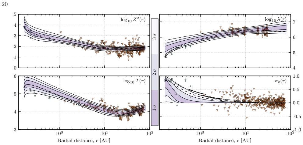
- [Section 3, footnote 3 and Eq. (11)] The error model is not coherent across variables. The footnote says the data and model estimates are base-10 log-transformed before χ² is computed, but σc and σD are signed and cannot be log-transformed; the paper does not specify which variables enter the χ² sum in which form. With k = 1 for all terms, Z², λ, and T are assigned an error of one decade, while σc and σD receive an absolute error of 1. This effectively downweights the σc and σD data by comparison. The σc mismatch visible in Figure 1 (observed values scattered between roughly ±0.5 beyond 1 AU while the model collapses to σc ≈ 0) is therefore not penalized as strongly as a comparable fractional mismatch in Z² or λ. Because the same σc data are used in every model comparison, this weighting can bias both parameter constraints and the Bayes factors; the authors should document the per-variable transformation and justify the relative weighting.
- [Section 4.4 and Table 5] The conclusion that pickup-ion effects in the λ equation are 'decisively favoured' is drawn from Δ ln K values that are close to the chosen threshold. For example, in the α-β-σD-fD-Csh case, the standard model has ln K = −4.35 and the no-λ-PI version has ln K = −9.70, giving Δ = 5.35. Because all of these values inherit the arbitrary k = 1 calibration, and because comparisons across models with different numbers of parameters include prior-volume terms that do not rescale with k in the same way as the likelihood term, the word 'decisive' is not supported. The qualitative direction of the comparison may survive with a more realistic error model—indeed it is physically plausible—but the strength of the claim needs to be recalibrated or rephrased as conditional on the assumed error model.
- [Section 6 and Table 1] The recommended parameter set 'α = 0.16 ± 0.03, β = 0.10 ± 0.02, the parameters stated in Table 1' does not correspond to a single analysis. Table 1 contains nominal values for σD, Csh, and fD (e.g., Csh = 1.5), while the full analyses in Section 4.2 report different posterior means (e.g., Csh ≈ 2 for the 2D α-β-BC-σD-fD-Csh case). Please specify which analysis the recommendation is drawn from and whether the other parameters should be fixed at their nominal values or at their posterior means; as written, the recommendation is internally inconsistent.
minor comments (5)
- [Section 2.3 and Table 2] Table 2 says the fixed inner boundary values are 'approximately those from PSP data presented in Adhikari et al. (2015)', but PSP was not operational in 2015; the intended reference is likely Adhikari et al. (2021). Please correct the citation.
- [Section 5.1.1 and Figure 7b] The method used to fit the linear relations α = mβ in the α–β plane is not described; please state the fitting procedure (e.g., weighted least squares on which variables) and report the uncertainties of the fitted slopes.
- [Section 4.1 and Figure 1] The paper notes the unphysical T(r) increase near the inner boundary and the systematic offset from PSP temperatures, but does not discuss whether removing the innermost radial bins would change the α–β posteriors; a brief sensitivity statement would be helpful.
- [Section 3] The sentence 'we therefore assume the error is constant and the same for all datapoints (i.e., σ_i = k is constant), and obtain an unnormalized likelihood function by setting k = 1' conflates two distinct choices: the shape of the error model (same for all points) and the numerical value k = 1. Readers would benefit from an explicit statement that the latter is a convention, not an estimate.
- [References] The reference 'Oughton & Bishop 2024' is listed as 'in Solar Wind 16, Vol. in preparation'; if it is now available or submitted, please update the citation.
Circularity Check
No load-bearing circularity: the Bayesian parameter estimates and model comparisons are standard fits to external PSP/Voyager data; the only self-citation is minor and non-load-bearing, and the arbitrary common error scale is an acknowledged limitation rather than a circular reduction.
full rationale
The paper's central output is a Bayesian posterior estimate of TTM parameters (alpha, beta, sigma_D, f_D, C_sh, and boundary conditions) from PSP and Voyager 2 radial profiles, together with Bayes-factor model comparisons. This is ordinary parameter estimation and model selection, not a derivation that returns its own inputs. The quoted recommendation, 'use of the 2D TTM with alpha = 0.16 +/- 0.03, beta = 0.10 +/- 0.02,' is explicitly the mean of a posterior distribution conditioned on the data and priors, so it is a fitted value honestly reported as a fit, not a prediction derived from first principles. The model-comparison step uses the same likelihood for all models, which is standard practice. The PI-term inclusion test ('no lambda PI' versus the standard equation) compares two distinct model forms and is a genuine model-selection exercise, even though the PI lambda term is derived from the conservation law Z^{2 beta/alpha} lambda = const; testing that term against data is not circular because the alternative model simply omits it. The paper's acknowledged limitation, 'Currently, we do not have measurements (or estimates) for the error of the datapoints sigma_i. We therefore assume the error is constant and the same for all datapoints (i.e., sigma_i = k is constant), and obtain an unnormalized likelihood function by setting k = 1,' indeed means the posterior widths and Bayes-factor magnitudes are conditioned on an arbitrary error scale, and the statement that Bayes factors with the same error assumptions 'should be defensible' is statistically fragile because ln K generally rescales with 1/k^2. However, this is a correctness/robustness concern about an untested hyperparameter, not a circular equation: the model outputs are not defined in terms of the recommended parameters, and the data are external to the fitted values. The only self-citation to prior work by the same authors (Oughton & Bishop 2024) appears as an aside about analytic solutions and is not load-bearing. The TTM itself is taken from Breech et al. (2008), a published external model that the paper corrects and then tests; using it as an input is not circular. Accordingly, no specific circular step can be exhibited, and the appropriate finding is no significant circularity, with a minor self-citation and an arbitrary error-scale caveat.
Assumptions & free parameters
free parameters (6)
- α (von Kármán–Howarth energy cascade coefficient) =
0.16 ± 0.03 (posterior mean, 2D recommended model)
- β (von Kármán–Howarth length cascade coefficient) =
0.10 ± 0.02 (posterior mean, 2D recommended model)
- σD (normalized residual energy, assumed constant) =
-0.36 to -0.38 (posterior means across extended analyses)
- fD (pickup-ion injection strength) =
≈0.12-0.2 depending on analysis
- Csh (stream shear driving coefficient) =
≈2-3 (posterior means in extended analyses)
- Z^2_0.17, λ_0.17, σc_0.17, T_0.17 (inner boundary conditions) =
Posterior distributions shown in Figure 2; means include Z^2_0.17 slightly above 7,040 (km/s)^2, λ_0.17 varying with…
assumptions (6)
- standard math Bayes theorem and nested sampling provide valid posterior inference and evidence estimation.
- domain assumption The 1D steady-state TTM equations (1)-(4) adequately describe solar wind turbulence between 0.17 and 80 AU.
- domain assumption Z^(2β/α) λ is locally conserved under pickup-ion driving.
- domain assumption σD is constant, with dσD/dr = 0.
- domain assumption All cascaded turbulence energy heats protons (α_T = 1) in the main results.
- domain assumption PSP and Voyager 2 binned averages are direct measurements of Z^2, λ, σc, σD, and T, with no associated uncertainties.
Cite this review
Pith. "Pith review of Constraining solar wind transport model parameters using Bayesian analysis." pith.science (2026). https://pith.science/paper/P6H537MB
@misc{pith2026241207897,
  author       = {Pith},
  title        = {Pith review of: Constraining solar wind transport model parameters using Bayesian analysis},
  year         = {2026},
  howpublished = {\url{https://pith.science/paper/P6H537MB}},
  note         = {Machine review of arXiv:2412.07897}
}
abstract
We apply nested-sampling (NS) Bayesian analysis [AshtonEA22] to a model for the transport of MHD-scale solar wind fluctuations. The dual objectives are to obtain improved constraints on parameters present in the turbulence transport model (TTM) and to support comparisons of distinct versions of the TTM. The TTMs analysed are essentially 1D steady-state presented in [BreechEA08] that describe the radial evolution of the energy, correlation length, and normalized cross helicity of the fluctuations, together with the proton temperature, in prescribed background solar wind fields. Modelled effects present in the TTM include nonlinear turbulence interactions, shear driving, and energy injection associated with pickup-ions. These effects involve adjustable parameters that we seek to constrain. Bayesian analysis supports the efficient searching of a parameter space for the 'best' set of TTM parameter values. More advanced use provides the parameter's posterior distribution: its probability given the data, and the model. This can be used to understand the uncertainty in the provided 'best' values for the parameters and therefore the uncertainty in the suggested TTM solutions/predictions. By using NS, we can calculate the Bayesian evidence for each TTM and objectively determine which best fits the given observational data. Based on the analysis of the datasets and TTM employed, we recommend use of the 2D TTM with von Karman-Howarth parameters ${\alpha}\approx 0.16$ and $\beta \approx 0.10$ and parameter assumptions from existing literature. It is important to include the pickup ion effects in the lengthscale evolution equation by assuming $Z^{2\beta/\alpha}\lambda = const$ is locally conserved. This work is readily extended to more sophisticated solar wind models. Although more work is required to generate datasets with associated errors, which is necessary for accurate Bayesian modelling.
Figures


Figures from the paper (9 more)



Reference graph
Works this paper leans on
-
[1]
, " * write output.state after.block = add.period write newline
ENTRY address archivePrefix author booktitle chapter doi edition editor eprint howpublished institution journal key month number organization pages publisher school series title misctitle type volume year version url label extra.label sort.label short.list INTEGERS output.state before.all mid.sentence after.sentence after.block FUNCTION init.state.consts ...
-
[2]
write newline
" write newline "" before.all 'output.state := FUNCTION format.url url empty "" new.block "" url * "" * if FUNCTION format.eprint eprint empty "" archivePrefix empty "" archivePrefix "arXiv" = new.block " " eprint * " " * new.block " " eprint * " " * if if if FUNCTION format.doi doi empty "" " " doi * " " * if FUNCTION format.pid doi empty eprint empty ur...
-
[3]
?pI5Jh .- /@H4&Tf:y r|Hh# N b#V ^U+
thebibliography [1] 20pt to REFERENCES 6pt =0pt -12pt 10pt plus 3pt =0pt =0pt =1pt plus 1pt =0pt =0pt -12pt =13pt plus 1pt =20pt =13pt plus 1pt \@M =10000 =-1.0em =0pt =0pt 0pt =0pt =1.0em @enumiv\@empty 10000 10000 `\.\@m \@noitemerr \@latex@warning Empty `thebibliography' environment \@ifnextchar \@reference \@latexerr Missing key on reference command E...
2021
-
[4]
, " * write output.state after.block = add.period write newline
ENTRY address author booktitle chapter doi edition editor eid howpublished institution journal key month note number organization pages publisher school series title type volume year label extra.label sort.label short.list INTEGERS output.state before.all mid.sentence after.sentence after.block FUNCTION init.state.consts #0 'before.all := #1 'mid.sentence...
-
[5]
write newline
" write newline "" before.all 'output.state := FUNCTION if.digit duplicate "0" = swap duplicate "1" = swap duplicate "2" = swap duplicate "3" = swap duplicate "4" = swap duplicate "5" = swap duplicate "6" = swap duplicate "7" = swap duplicate "8" = swap "9" = or or or or or or or or or FUNCTION n.separate 't := "" #0 'numnames := t empty not t #-1 #1 subs...
-
[6]
Abbott, T. M. C., Allam, S., Andersen, P., et al. 2019, The Astrophysical Journal, 872, L30, 10.3847/2041-8213/ab04fa
-
[7]
Adhikari, L., Zank, G. P., Bruno, R., et al. 2015, Astrophys.\ J., 805, 63, 10.1088/0004-637X/805/1/63
-
[8]
Adhikari, L., Zank, G. P., Hunana, P., et al. 2017 a , Astrophys.\ J., 841, 85, 10.3847/1538-4357/aa6f5d
Show all 122 references
-
[9]
P., Telloni, D., et al
Adhikari, L., Zank, G. P., Telloni, D., et al. 2017 b , Astrophys.\ J., 851, 117, 10.3847/1538-4357/aa9ce4
2017 doi
- [10]
-
[11]
P., Wang, B., et al
Adhikari, L., Zank, G. P., Wang, B., et al. 2023, Astrophys.\ J., 953, 44, 10.3847/1538-4357/acde57
2023 doi
-
[12]
2022, Nature Reviews Methods Primers, 2, 39, 10.1038/s43586-022-00121-x
Ashton, G., Bernstein, N., Buchner, J., et al. 2022, Nature Reviews Methods Primers, 2, 39, 10.1038/s43586-022-00121-x
2022 doi
-
[13]
H., Oughton, S., & Wan, M
Bandyopadhyay, R., Matthaeus, W. H., Oughton, S., & Wan, M. 2019, J.\ Fluid Mech., 876, 5, 10.1017/jfm.2019.513
2019 doi
-
[14]
2018, Phys.\ Rev.\ X, 8, 041052, 10.1103/PhysRevX.8.041052
Bandyopadhyay, R., Oughton, S., Wan, M., et al. 2018, Phys.\ Rev.\ X, 8, 041052, 10.1103/PhysRevX.8.041052
2018 doi
-
[15]
M., Matthaeus, W
Bandyopadhyay, R., Meyer, C. M., Matthaeus, W. H., et al. 2023, Astrophys.\ J. Lett., 955, L28, 10.3847/2041-8213/acf85e
2023 doi
-
[16]
2021, Astrophysics Source Code Library, ascl:2103.022
Barbary, K. 2021, Astrophysics Source Code Library, ascl:2103.022
2021
-
[17]
W., & Davis Jr., L
Belcher, J. W., & Davis Jr., L. 1971, J.\ Geophys.\ Res., 76, 3534, 10.1029/JA076i016p03534
1971 doi
-
[18]
W., Wanner, W., & Matthaeus, W
Bieber, J. W., Wanner, W., & Matthaeus, W. H. 1996, J.\ Geophys.\ Res., 101, 2511, 10.1029/95JA02588
1996 doi
-
[19]
H., Cranmer, S
Breech, B., Matthaeus, W. H., Cranmer, S. R., Kasper, J. C., & Oughton, S. 2009, J.\ Geophys.\ Res., 114, 10.1029/2009JA014354
2009 doi
-
[20]
H., Minnie, J., et al
Breech, B., Matthaeus, W. H., Minnie, J., et al. 2008, J.\ Geophys.\ Res., 113, 10.1029/2007JA012711
2008 doi
-
[21]
2005, Geophys.\ Res.\ Lett., 32, L06103, doi:10.1029/2004GL022321, 10.1029/2004GL022321
---. 2005, Geophys.\ Res.\ Lett., 32, L06103, doi:10.1029/2004GL022321, 10.1029/2004GL022321
2005 doi
-
[22]
J., P \'a rtay, L
Brewer, B. J., P \'a rtay, L. B., & Cs \'a nyi, G. 2010, Astrophysics Source Code Library, ascl:1010.029
2010
-
[23]
2013, Living Rev.\ Solar Phys., 10, 10.12942/lrsp-2013-2
Bruno, R., & Carbone, V. 2013, Living Rev.\ Solar Phys., 10, 10.12942/lrsp-2013-2
2013 doi
-
[24]
2016, Astrophysics Source Code Library, ascl:1606.005
Buchner, J. 2016, Astrophysics Source Code Library, ascl:1606.005
2016
-
[25]
2021, The Journal of Open Source Software, 6, 3001, 10.21105/joss.03001
---. 2021, The Journal of Open Source Software, 6, 3001, 10.21105/joss.03001
2021 doi
-
[26]
Burlaga, L. F. 1974, J.\ Geophys.\ Res., 79, 3717, 10.1029/JA079i025p03717
1974 doi
-
[27]
1990, Geophys.\ Astrophys.\ Fluid Dyn., 52, 153, 10.1080/03091929008219845
Carbone, V., & Veltri, P. 1990, Geophys.\ Astrophys.\ Fluid Dyn., 52, 153, 10.1080/03091929008219845
1990 doi
-
[28]
2014, Astronomy and Astrophysics, 571, A71, 10.1051/0004-6361/201424181
Corsaro, E., & De Ridder, J. 2014, Astronomy and Astrophysics, 571, A71, 10.1051/0004-6361/201424181
2014 doi
-
[29]
Cranmer, S. R. 2009, Living Rev.\ Solar Phys., 6. http://www.livingreviews.org/lrsp-2009-3
2009
-
[30]
R., Matthaeus, W
Cranmer, S. R., Matthaeus, W. H., Breech, B. A., & Kasper, J. C. 2009, Astrophys.\ J., 702, 1604, 10.1088/0004-637X/702/2/1604
2009 doi
-
[31]
E., Parashar, T
Cuesta, M. E., Parashar, T. N., Chhiber, R., & Matthaeus, W. H. 2022 a , Astrophys.\ J.\ Suppl. Ser, 259, 23, 10.3847/1538-4365/ac45fa
2022 doi
-
[32]
E., Chhiber, R., Roy, S., et al
Cuesta, M. E., Chhiber, R., Roy, S., et al. 2022 b , Astrophys.\ J. Lett., 932, L11, 10.3847/2041-8213/ac73fd
2022 doi
-
[33]
Dryden, H. L. 1943, Quart.\ Appl.\ Math., 1, 7, 10.1090/qam/8209
1943 doi
-
[34]
A., McComas, D
Elliott, H. A., McComas, D. J., Zirnstein, E. J., et al. 2019, The Astrophysical Journal, 885, 156, 10.3847/1538-4357/ab3e49
2019 doi
-
[35]
Ellison, A. M. 2004, Ecology Letters, 7, 509, https://doi.org/10.1111/j.1461-0248.2004.00603.x
2004
-
[36]
E., Effenberger, F., Florinski, V., et al
Engelbrecht, N. E., Effenberger, F., Florinski, V., et al. 2022, Space Sci Rev, 218, 33, 10.1007/s11214-022-00896-1
2022 doi
-
[37]
Feroz, F., & Hobson, M. P. 2008, Monthly Notices of the Royal Astronomical Society, 384, 449, 10.1111/j.1365-2966.2007.12353.x
2008
-
[38]
P., & Bridges, M
Feroz, F., Hobson, M. P., & Bridges, M. 2009, Monthly Notices of the Royal Astronomical Society, 398, 1601, 10.1111/j.1365-2966.2009.14548.x
2009
-
[39]
2022, Space Sci.\ Rev., 218, 50, 10.1007/s11214-022-00914-2
Fraternale, F., Adhikari, L., Fichtner, H., et al. 2022, Space Sci.\ Rev., 218, 50, 10.1007/s11214-022-00914-2
2022 doi
-
[40]
1997, Astrophys.\ J., 485, 680, 10.1086/304442
Goldreich, P., & Sridhar, S. 1997, Astrophys.\ J., 485, 680, 10.1086/304442
1997 doi
-
[41]
2018, The Journal of Open Source Software, 3, 849, 10.21105/joss.00849
Handley, W. 2018, The Journal of Open Source Software, 3, 849, 10.21105/joss.00849
2018 doi
-
[42]
J., Hobson, M
Handley, W. J., Hobson, M. P., & Lasenby, A. N. 2015, Monthly Notices of the Royal Astronomical Society, 453, 4384, 10.1093/mnras/stv1911
2015 doi
-
[43]
M., S tver \'a k , v., Matteini, L., & Velli, M
Hellinger, P., Tr \'a vn\' c ek , P. M., S tver \'a k , v., Matteini, L., & Velli, M. 2013, J.\ Geophys.\ Res., 118, 1351, 10.1002/jgra.50107
2013 doi
-
[44]
2011, Journal of Cosmology and Astroparticle Physics, 2011, 005, 10.1088/1475-7516/2011/08/005
Hojjati, A., Pogosian, L., & Zhao, G.-B. 2011, Journal of Cosmology and Astroparticle Physics, 2011, 005, 10.1088/1475-7516/2011/08/005
2011 doi
-
[45]
C., Pontius Jr., D
Hossain, M., Gray, P. C., Pontius Jr., D. H., Matthaeus, W. H., & Oughton, S. 1995, Phys.\ Fluids, 7, 2886, 10.1063/1.868665
1995 doi
-
[46]
Howes, G. G. 2011, Astrophys.\ J., 738, 40, 10.1088/0004-637X/738/1/40
2011 doi
-
[47]
L., & Li, H
Huang, Y., Shao, C., Wu, B., Beck, J. L., & Li, H. 2019, Advances in Structural Engineering, 22, 1329, 10.1177/1369433218811540
2019 doi
-
[48]
Isenberg, P. A. 2005, Astrophys.\ J., 623, 502, 10.1086/428609
2005 doi
-
[49]
A., Smith, C
Isenberg, P. A., Smith, C. W., & Matthaeus, W. H. 2003, Astrophys.\ J., 592, 564, 10.1086/375584
2003 doi
-
[50]
A., Smith, C
Isenberg, P. A., Smith, C. W., Matthaeus, W. H., & Richardson, J. D. 2010, Astrophys.\ J., 719, 716, 10.1088/0004-637X/719/1/716
2010 doi
-
[51]
C., Rumsey, C., & Saunders, R
Javid, K., Perrott, Y. C., Rumsey, C., & Saunders, R. D. E. 2019, Monthly Notices of the Royal Astronomical Society, 489, 3135, 10.1093/mnras/stz2341
2019 doi
-
[52]
H., & Jeffreys, S
Jeffreys, S. H., & Jeffreys, S. H. 1998, The Theory of Probability , third edition, third edition edn., Oxford Classic Texts in the Physical Sciences ( Oxford, New York : Oxford University Press )
1998
-
[53]
Jungman, G., Kamionkowski, M., Kosowsky, A., & Spergel, D. N. 1996, Physical Review D, 54, 1332, 10.1103/PhysRevD.54.1332
1996 doi
- [54]
-
[55]
2023, Astrophys.\ J., 953, 133, 10.3847/1538-4357/acd84e
Kleimann, J., Oughton, S., Fichtner, H., & Scherer, K. 2023, Astrophys.\ J., 953, 133, 10.3847/1538-4357/acd84e
2023 doi
-
[56]
Kolmogorov, A. N. 1941, C.R. Acad. Sci. U.R.S.S., 31, 538
1941
-
[57]
1987, J.\ Geophys.\ Res., 92, 11041, 10.1029/JA092iA10p11041
Lee, M., & Ip, W.-H. 1987, J.\ Geophys.\ Res., 92, 11041, 10.1029/JA092iA10p11041
1987 doi
- [58]
-
[59]
Linkmann, M., Berera, A., & Goldstraw, E. E. 2017, Phys.\ Rev.\ E, 95, 013102, 10.1103/PhysRevE.95.013102
2017 doi
-
[60]
H., Ghosh, S., Oughton, S., & Roberts, D
Matthaeus, W. H., Ghosh, S., Oughton, S., & Roberts, D. A. 1996 a , J.\ Geophys.\ Res., 101, 7619, 10.1029/95JA03830
1996 doi
-
[61]
H., Goldstein, M
Matthaeus, W. H., Goldstein, M. L., & Roberts, D. A. 1990, J.\ Geophys.\ Res., 95, 20\,673, 10.1029/JA095iA12p20673
1990 doi
-
[62]
H., Oughton, S., Pontius, D., & Zhou, Y
Matthaeus, W. H., Oughton, S., Pontius, D., & Zhou, Y. 1994, J.\ Geophys.\ Res., 99, 19\,267, 10.1029/94JA01233
1994 doi
-
[63]
H., Zank, G
Matthaeus, W. H., Zank, G. P., & Oughton, S. 1996 b , J.\ Plasma Phys., 56, 659, 10.1017/S0022377800019516
1996 doi
-
[64]
H., Zank, G
Matthaeus, W. H., Zank, G. P., Smith, C. W., & Oughton, S. 1999, Phys.\ Rev.\ Lett., 82, 3444, 10.1103/PhysRevLett.82.3444
1999 doi
-
[65]
2019, The Astrophysical Journal, 884, 145
McComas, D., Rankin, J., Schwadron, N., & Swaczyna, P. 2019, The Astrophysical Journal, 884, 145
2019
-
[66]
E., Mc Comas , D
Neugebauer, M., Goldstein, B. E., Mc Comas , D. J., Suess, S. T., & Balogh, A. 1995, J.\ Geophys.\ Res., 100, 23\,389, 10.1029/95JA02723
1995 doi
-
[67]
Oughton, S., & Bishop, M. A. 2024, in Solar Wind 16, Vol. in preparation
2024
-
[68]
Oughton, S., & Engelbrecht, N. E. 2021, New Astron., 83, 10.1016/j.newast.2020.101507
2021
-
[69]
Oughton, S., & Matthaeus, W. H. 2020, Astrophys.\ J., 897, 10.3847/1538-4357/ab8f2a
2020 doi
-
[70]
H., Smith, C
Oughton, S., Matthaeus, W. H., Smith, C. W., Breech, B., & Isenberg, P. A. 2011, J.\ Geophys.\ Res., 116, 10.1029/2010JA016365
2011 doi
-
[71]
H., Wan, M., & Osman, K
Oughton, S., Matthaeus, W. H., Wan, M., & Osman, K. T. 2015, Phil.\ Trans.\ R.\ Soc.\ A, 373, 10.1098/rsta.2014.0152
2015
-
[72]
R., & Matthaeus, W
Oughton, S., Priest, E. R., & Matthaeus, W. H. 1994, J.\ Fluid Mech., 280, 95, 10.1017/S0022112094002867
1994 doi
-
[73]
N., Cuesta, M., & Matthaeus, W
Parashar, T. N., Cuesta, M., & Matthaeus, W. H. 2019, Astrophys.\ J., 884, L57, 10.3847/2041-8213/ab4a82
2019 doi
-
[74]
Parker, E. N. 1958, Astrophys.\ J., 128, 664, 10.1086/146579
1958 doi
-
[75]
1965, Space Sci.\ Rev., 4, 666, 10.1007/BF00216273
---. 1965, Space Sci.\ Rev., 4, 666, 10.1007/BF00216273
1965 doi
-
[76]
Parkinson, D., & Liddle, A. R. 2013, Statistical Analysis and Data Mining: The ASA Data Science Journal, 9, 3, 10.1002/sam.11179
2013 doi
-
[77]
2011, Astrophysics Source Code Library, ascl:1110.019
Parkinson, D., Mukherjee, P., & Liddle, A. 2011, Astrophysics Source Code Library, ascl:1110.019
2011
-
[78]
W., Breech, B., et al
Pei, C., Bieber, J. W., Breech, B., et al. 2010, J.\ Geophys.\ Res., 115, 10.1029/2009JA014705
2010 doi
-
[79]
R., Goldhaber, G., et al
Perlmutter, S., Pennypacker, C. R., Goldhaber, G., et al. 1995, The Astrophysical Journal, 440, L41, 10.1086/187756
1995 doi
-
[80]
2010, Geophys.\ Res.\ Lett., 37, 10.1029/2010GL044570
Perri, S., & Balogh, A. 2010, Geophys.\ Res.\ Lett., 37, 10.1029/2010GL044570
2010 doi
-
[81]
C., Javid, K., Carvalho, P., et al
Perrott, Y. C., Javid, K., Carvalho, P., et al. 2019, Monthly Notices of the Royal Astronomical Society, 486, 2116, 10.1093/mnras/stz826
2019 doi
-
[82]
1983, SIAM Journal on Scientific and Statistical Computing, 4, 136, 10.1137/0904010
Petzold, L. 1983, SIAM Journal on Scientific and Statistical Computing, 4, 136, 10.1137/0904010
1983 doi
-
[83]
2020, Astronomy and Astrophysics, 641, A6, 10.1051/0004-6361/201833910
Planck Collaboration , Aghanim, N., Akrami, Y., et al. 2020, Astronomy and Astrophysics, 641, A6, 10.1051/0004-6361/201833910
2020 doi
-
[84]
V., Arge, C
Pogorelov, N. V., Arge, C. N., Caplan, R. M., et al. 2024, J. Phys.: Conf. Ser., 2742, 012013, 10.1088/1742-6596/2742/1/012013
2024 doi
-
[85]
D., & Smith, C
Richardson, J. D., & Smith, C. W. 2003, Geophys.\ Res.\ Lett., 30, 1206, doi:10.1029/2002GL016551, 10.1029/2002GL016551
2003 doi
-
[87]
Schekochihin, A. A. 2022, J.\ Plasma Phys., 88, 155880501, 10.1017/S0022377822000721
2022 doi
- [88]
-
[89]
2017, Annual Review of Astronomy and Astrophysics, 55, 213, 10.1146/annurev-astro-082214-122339
Sharma, S. 2017, Annual Review of Astronomy and Astrophysics, 55, 213, 10.1146/annurev-astro-082214-122339
2017 doi
-
[90]
V., Matthaeus, W
Shebalin, J. V., Matthaeus, W. H., & Montgomery, D. 1983, J.\ Plasma Phys., 29, 525, 10.1017/S0022377800000933
1983 doi
-
[91]
P., Adhikari, L., et al
Shiota, D., Zank, G. P., Adhikari, L., et al. 2017, Astrophys.\ J., 837, 75, 10.3847/1538-4357/aa60bc
2017 doi
-
[92]
Skilling, J. 2004, in BAYESIAN INFERENCE AND MAXIMUM ENTROPY METHODS IN SCIENCE AND ENGINEERING: 24th International Workshop on Bayesian Inference and Maximum Entropy Methods in Science and Engineering, Vol. 735 (AIP), 395--405, 10.1063/1.1835238
2004 doi
-
[94]
W., Matthaeus, W
Smith, C. W., Matthaeus, W. H., Zank, G. P., et al. 2001, J.\ Geophys.\ Res., 106, 8253, 10.1029/2000JA000366
2001 doi
-
[95]
W., & Vasquez, B
Smith, C. W., & Vasquez, B. J. 2024, Front. Astron. Space Sci., 11, 10.3389/fspas.2024.1371058
2024
-
[96]
W., Vasquez, B
Smith, C. W., Vasquez, B. J., & Hamilton, K. 2006 b , J.\ Geophys.\ Res., 111, A09111, doi:10.1029/2006JA011651, 10.1029/2006JA011651
2006 doi
-
[97]
J., & Wolfe, J
Smith, E. J., & Wolfe, J. H. 1976, Geophys.\ Res.\ Lett., 3, 137, 10.1029/GL003i003p00137
1976 doi
-
[98]
M., Kucharek, H., Baliukin, I
Sok \'o , J. M., Kucharek, H., Baliukin, I. I., et al. 2022, Space Sci Rev, 218, 18, 10.1007/s11214-022-00883-6
2022 doi
-
[99]
Speagle, J. S. 2020, Monthly Notices of the Royal Astronomical Society, 493, 3132, 10.1093/mnras/staa278
2020 doi
-
[101]
2008, Contemporary Physics, 49, 71, 10.1080/00107510802066753
Trotta, R. 2008, Contemporary Physics, 49, 71, 10.1080/00107510802066753
2008 doi
-
[102]
1987, Solar Phys., 109, 149, 10.1086/498671
Tu, C. 1987, Solar Phys., 109, 149, 10.1086/498671
1987 doi
-
[103]
1995, Space Sci.\ Rev., 73, 1, 10.1007/BF00748891
Tu, C.-Y., & Marsch, E. 1995, Space Sci.\ Rev., 73, 1, 10.1007/BF00748891
1995 doi
-
[104]
1984, J.\ Geophys.\ Res., 89, 9695, 10.1029/JA089iA11p09695
Tu, C.-Y., Pu, Z.-Y., & Wei, F.-S. 1984, J.\ Geophys.\ Res., 89, 9695, 10.1029/JA089iA11p09695
1984 doi
-
[105]
H., Breech, B
Usmanov, A., Matthaeus, W. H., Breech, B. A., & Goldstein, M. L. 2011, Astrophys.\ J., 727, 84, 10.1088/0004-637X/727/2/84
2011 doi
-
[106]
V., Goldstein, M
Usmanov, A. V., Goldstein, M. L., & Matthaeus, W. H. 2014, Astrophys.\ J., 788, 43, 10.1088/0004-637X/788/1/43
2014 doi
-
[107]
2016, Astrophys.\ J., 820, 17, 10.3847/0004-637X/820/1/17
---. 2016, Astrophys.\ J., 820, 17, 10.3847/0004-637X/820/1/17
2016 doi
-
[108]
V., Matthaeus, W
Usmanov, A. V., Matthaeus, W. H., Goldstein, M. L., & Chhiber, R. 2018, Astrophys.\ J., 865, 25, 10.3847/1538-4357/aad687
2018 doi
-
[109]
2021, Nature Reviews Methods Primers, 1, 1
van de Schoot, R., Depaoli, S., King, R., et al. 2021, Nature Reviews Methods Primers, 1, 1
2021
-
[110]
V., Meng, X., et al
van der Holst , B., Sokolov, I. V., Meng, X., et al. 2014, Astrophys.\ J., 782, 81, 10.1088/0004-637X/782/2/81
2014 doi
-
[111]
1989, Phys.\ Rev.\ Lett., 63, 1807, 10.1103/PhysRevLett.63.1807
Velli, M., Grappin, R., & Mangeney, A. 1989, Phys.\ Rev.\ Lett., 63, 1807, 10.1103/PhysRevLett.63.1807
1989 doi
- [112]
-
[113]
Wan, M., Oughton, S., Servidio, S., & Matthaeus, W. H. 2012, J.\ Fluid Mech., 697, 296, 10.1017/jfm.2012.61
2012 doi
-
[114]
2003, Journal of Geophysical Research: Space Physics, 108, https://doi.org/10.1029/2002JA009322
Wang, C., & Richardson, J. 2003, Journal of Geophysical Research: Space Physics, 108, https://doi.org/10.1029/2002JA009322
2003 doi
-
[115]
2015, Astrophys.\ J., 805, 155, 10.1088/0004-637X/805/2/155
Wiengarten, T., Fichtner, H., Kleimann, J., & Kissmann, R. 2015, Astrophys.\ J., 805, 155, 10.1088/0004-637X/805/2/155
2015 doi
-
[116]
E., et al
Wiengarten, T., Oughton, S., Engelbrecht, N. E., et al. 2016, Astrophys.\ J., 833, 17, 10.3847/0004-637X/833/1/17
2016 doi
-
[117]
L., & Zank, G
Williams, L. L., & Zank, G. P. 1994, J.\ Geophys.\ Res., 99, 19\,229, 10.1029/94JA01657
1994 doi
-
[118]
N., Oughton, S., de Lange, K., & Frean, M
Wrench, D., Parashar, T. N., Oughton, S., de Lange, K., & Frean, M. 2024, Astrophys.\ J., 961, 182, 10.3847/1538-4357/ad118e
2024 doi
-
[119]
2008, J.\ Turb., 9, 1, 10.1080/14685240802433057
Yokoi, N., Rubinstein, R., Hamba, F., & Yoshizawa, A. 2008, J.\ Turb., 9, 1, 10.1080/14685240802433057
2008 doi
-
[120]
P., Adhikari, L., Hunana, P., et al
Zank, G. P., Adhikari, L., Hunana, P., et al. 2017, Astrophys.\ J., 835, 147, 10.3847/1538-4357/835/2/147
2017 doi
-
[121]
P., Adhikari, L., Zhao, L.-L., et al
Zank, G. P., Adhikari, L., Zhao, L.-L., et al. 2018, Astrophys.\ J., 869, 23, 10.3847/1538-4357/aaebfe
2018 doi
-
[122]
P., Dosch, A., Hunana, P., et al
Zank, G. P., Dosch, A., Hunana, P., et al. 2012, Astrophys.\ J., 745, 35, 10.1088/0004-637X/745/1/35
2012 doi
-
[123]
P., Matthaeus, W
Zank, G. P., Matthaeus, W. H., & Smith, C. W. 1996, J.\ Geophys.\ Res., 101, 17\,093, 10.1029/96JA01275
1996 doi
-
[124]
Zhou, Y., & Matthaeus, W. H. 1990, J.\ Geophys.\ Res., 95, 10\,291, 10.1029/JA095iA07p10291
1990 doi
-
[125]
J., M \"o bius, E., Zhang, M., et al
Zirnstein, E. J., M \"o bius, E., Zhang, M., et al. 2022, Space Sci Rev, 218, 28, 10.1007/s11214-022-00895-2
2022 doi
Reviewed August 11, 2026 · model on record in the stance chip above.
Discussion (0). Continue with ORCID to comment.