REVIEW 4 major objections 6 minor 1 cited by
Generalized Bayesian deep reinforcement learning
T0 review · 4 major / 6 minor · reviewed 2026-08-11 · deepseek-v4-flash
Pith's one-line read The paper establishes that Thompson sampling works for model-based RL with deep generative dynamics and no likelihood, via a prequential scoring-rule posterior that provably concentrates and turns Gaussian, plus a bound for expected…
desk verdict Promising likelihood-free Thompson sampling framework, but the BvM and ETS bounds rest on stationarity/mixing assumptions that the adaptive greedy-policy algorithm doesn't guarantee. read the letter →
The pith
A machine-rendered reading of the paper's core claim, the machinery that carries it, and where it could break.
The reading
What carries the argument
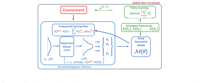
The load-bearing object is the prequential scoring-rule posterior, formed by exponentiating the negative cumulative one-step-ahead score instead of the log-likelihood; with the log score it reduces exactly to the usual likelihood posterior. The paper uses the energy score, a strictly proper scoring rule that can be estimated unbiasedly from simulator draws, and decomposes the prequential score by action to obtain a uniform law of large numbers under mixing assumptions. Posterior sampling uses sequential Monte Carlo with an adjusted stochastic-gradient Riemannian Langevin dynamics kernel, which handles the unbiased but noisy score gradients and scales to neural-network parameter spaces. Expected Thompson sampling then replaces the single posterior draw of classical Thompson sampling with an average of Q-functions over $n$ posterior samples, reducing estimation variance and, via the Bernstein–von Mises theorem, making the Q-approximation error contract.
What would settle it
Run a known parametric MDP with the prequential energy-score posterior while updating the policy every episode, and check whether the empirical distribution of states visited under each action converges as episodes accumulate and whether $\sqrt{T}(\theta-\hat\theta_T)$ is approximately Gaussian around the true parameter; if the visited-state distribution keeps drifting under a changing policy, the mixing and stationarity assumptions fail and the Bernstein–von Mises conclusion should not hold.
Extended reading notes
Core claim
On its own terms, the paper's claim is that the prequential scoring rule posterior $$\pi_{\mathrm{PS}}(\$\theta$\,|\,h_T) \propto \pi(\$\theta$)\exp\{-\mathrm{PS}_T(\$\theta$)\},$$ with $\mathrm{PS}_T(\theta)=\sum_{t=1}^{T} S(P_\theta(\cdot|s_t,a_t),s_{t+1})$ for a strictly proper scoring rule $S$, is a sound replacement for the intractable likelihood posterior of an MDP. Theorem 5 states that, under assumptions A1–A10, the minimizer $\hat\theta_T$ of the prequential score is consistent for $\theta^*$, the posterior concentrates at $\theta^*$, and the density of $\sqrt{T}(\theta-\hat\theta_T)$ converges in total variation to $\mathcal{N}(0,H_*^{-1})$; $H_*$ plays the role of the Fisher information matrix. Theorem 6 bounds the ETS policy-iteration error by $\gamma^j\|Q^*-Q^{\theta^{(k)}}_{\mu_1}\|_\infty + \sum_{l=1}^j \gamma^{j-l+1}\zeta_l(k,n)$, where $\zeta_l(k,n)$ vanishes as episodes $k$ and posterior samples $n$ grow. The paper further shows empirically that ETS with a prequential posterior learns a balancing policy faster than model-free LSPI on a well-specified and a misspecified inverted pendulum, and that ETS-integrated REINFORCE outperforms model-free REINFORCE on the Hopper benchmark.
Load-bearing premise
The load-bearing premise is that, under the agent's actual adaptive policy, the sequence of visited states becomes stationary and mixing fast enough with bounded moments; if the policy keeps changing as data accumulate, that is not automatic and is never verified in the experiments.
Editorial extensions
If this is right
- A generative neural network for environment dynamics can be used for principled Bayesian exploration without a likelihood, since only forward simulation and score gradients are needed.
- As interaction length grows, the generalized posterior behaves like a Gaussian centered at the prequential-score minimizer, so posterior uncertainty quantification and Thompson-style exploration inherit familiar asymptotic guarantees.
- Averaging Q-functions over $n$ posterior samples cuts the posterior-sampling component of the value-approximation error by a factor of about $\sqrt{n}$ relative to single-sample Thompson sampling.
- In the well-specified discrete-action case, ETS policy iteration contracts toward the optimal Q-function as episodes and samples grow.
- In the misspecified and continuous-action cases studied, ETS improves sample efficiency over model-free baselines, though without the paper's theoretical guarantees.
Reading between the lines
- Reading from the paper's assumptions, the mixing and asymptotic-stationarity conditions (A2–A3) are not automatic when policies are updated every episode from accumulated data, and they are not checked in the pendulum and Hopper experiments; the Bernstein–von Mises guarantee should be read as holding for a stabilized or sufficiently slowly adapting policy unless verified.
- When the generative model is misspecified, $\theta^*$ is the best one-step-ahead predictive proxy rather than the true dynamics; ETS will then explore around a proxy that may be poor for long-horizon planning, so a fair comparison would need to measure regret against the true environment rather than only against the fitted model.
- A testable extension is to compute the effective sample size of the SMC particles and compare regret across the number of posterior samples $n$; if the posterior is multimodal or poorly mixed, increasing $n$ may not reduce the ETS error as Theorem 6 predicts.
- The continuous-action ETS extension with REINFORCE is empirical; an actor-critic variant using the same prequential posterior could make the sample-efficiency gain available to high-dimensional action spaces.
Signed reviews
Editorial analysis
A structured set of objections, weighed in public.
Referee Report
Summary. The paper proposes a generalized Bayesian framework for model-based reinforcement learning in which the environment is a parametric Markov decision process with an intractable likelihood, modeled by a deep generative network. A prequential scoring rule posterior proportional to the prior times exp(-PS_T(theta)) is introduced, sampled via sequential Monte Carlo with an adjusted stochastic gradient Riemannian Langevin kernel. The authors prove a uniform law of large numbers, consistency of the prequential score minimizer, and a Bernstein-von Mises theorem under assumptions A1-A10, then derive an error bound for expected Thompson sampling in Theorem 6. Experiments on a chain task, inverted pendulum (well-specified and misspecified), and Hopper show sample-efficiency gains over model-free baselines, with the continuous-action Hopper extension explicitly lacking theoretical guarantees.
Significance. If fully established, the framework would provide a useful likelihood-free posterior inference recipe for simulator-based MDPs and a multi-sample Thompson sampling scheme with a formal value-function error bound. The paper is transparent that the continuous-action extension and the misspecified deep generative models fall outside the stated theoretical conditions. The main weaknesses are that the central asymptotic results are stated for an adaptively updated, greedy policy while the stationarity and mixing assumptions are neither verified nor automatic, and that the ETS rate argument in Appendix B contains a gap. These issues are substantive but appear addressable by restricting the theoretical claims to settings where A2/A3 hold or by proving them under an explicit exploration scheme.
major comments (4)
- [Section 3.2, Assumptions A2/A3 and Lemma 2] The ULLN in Lemma 2 is the basis for Corollary 3, Lemma 4, and Theorem 5, and it relies on Assumptions A2/A3 for the process generated under the agent's policy. In Algorithm 1, however, the policy is updated after every episode from accumulated data and is then played greedily, so the action at time t depends on the whole history. For such an adaptive policy sequence, the Cesaro limit in A2 need not exist, the sets T_a may fail to grow for actions that become suboptimal once the policy converges, and conditioning on the event A_t=a can destroy the mixing property even when the environment M0 is Markovian. The statement following Lemma 2 that these properties hold automatically for the Markovian model M0 is therefore too strong. No verification of A2/A3 is supplied for the chain, pendulum, or Hopper experiments, so Theorem 5 is not established for the episodic adaptive setting that the algorithm actually implements.
- [Appendix B, Eq. (26) and following paragraph] The proof of Theorem 6 defines Y_ki = ||theta_ki - hat_theta_k|| + ||hat_theta_k - theta*|| and claims that (1/n) sum_{i=1}^n |Y_ki| = O_p((n k tau)^{-1/2}). This does not follow from the BvM result: each Y_ki is nonnegative and of stochastic order (k tau)^{-1/2}, so averaging n such terms does not reduce the order below the mean unless the terms are centered at zero, which they are not. Thus the claimed sqrt(n) improvement of ETS over classical TS is not proven by this argument. In addition, the assertion that the policy-iteration difference terms ||Q^{theta*}_{mu*_j} - Q^{theta*}_{mu_j}|| and ||Q^{theta*}_{mu*_{j+1}} - Q^{theta*}_{mu_{j+1}}|| vanish 'from the consistency of the posterior mean' requires that the greedy policies under Q^{theta*} and Q^{theta(k)} eventually coincide; this stability property does not follow from the BvM theorem alone and is not proved in the appendix.
- [Section 5.1, misspecified paragraph; Theorem 5 assumptions] The text states that Theorem 5 and Theorem 6 'assume an unimodal posterior for model parameters'. Global unimodality is not among assumptions A1-A10, and a Bernstein-von Mises theorem is a local result; if unimodality is intended as an additional condition, it must be stated where the theorems are proved. More importantly, the misspecified inverted-pendulum experiment and the Hopper experiment use generative neural networks whose posteriors the authors themselves describe as possibly multimodal, so the demonstrations involving deep generative models are not covered by the conditions under which Theorem 5 and Theorem 6 are claimed. This limitation should be made explicit in the theorem statements or in the theory section.
- [Appendix A.5, Theorem 5 proof] The proof of Theorem 5 is a sketch that imports Theorems 4 and 6 of Miller (2021). This is acceptable only if the imported hypotheses are verified. In particular, Assumption A8 requires PS''_T(theta*) to converge to a positive definite H*, and Assumption A10 requires a uniform separation of the empirical prequential score outside shrinking neighborhoods of hat_theta_T; these are substantive conditions on a simulator-based loss and are neither derived from the assumed generative model class nor checked in the experiments. The statement that q_T converges 'almost surely' also needs a precise formulation, since q_T is the density of a random probability measure and the total-variation convergence should be phrased as almost sure convergence of that random measure under M0, matching the formulation in Miller (2021).
minor comments (6)
- [Section 3.2, Assumption A2] The notation '1/|T_a| G^a_t converges weakly' is ambiguous; the intended statement is that the Cesaro average (1/|T_a|) sum_{t in T_a} G^a_t converges weakly to G^a, and the condition |T_a| -> infinity should be stated explicitly.
- [Theorem 5 statement] There is a typo in 'pospteerior', and in the normalizing-constant formula exp(-PS_T(theta_T)) the symbol theta_T appears to be a typo for hat_theta_T.
- [Appendix A.3, Eq. (19)] In Eq. (19) the notation gPS(theta) is missing the subscript T, and the bound epsilon T / 2 should be justified with the T-normalization made explicit when it is used in the following display.
- [Appendix C.2] The zeroth-order gradient formula appears to contain a typo: the second bracket should be [U(theta + mu z_i) - U(theta)] rather than [U(theta + mu z_i) - f(theta)].
- [Appendix B] The Lipschitz constant K'_mu = max_{(s,a) in S x A} K_mu(s,a) is used without a uniform bound over the policies generated by policy iteration; a uniform bound over the relevant policy class is needed for the recursion to be meaningful.
- [References and Section 5.2] The reference to Pacchiardi et al. (2024a) contains the typo 'Journal of Mahcine Learning Research', and the Hopper experiment would benefit from reporting the total number of episodes and the number of seeds used beyond the moving-average plot in Fig. 6.
Circularity Check
No significant circularity: BvM is an application of Miller (2021) to the prequential scoring-rule posterior, and the ETS bound is a Bellman-contraction inequality; self-citations to Pacchiardi et al. are external published support.
full rationale
The derivation chain is not circular. The prequential scoring-rule posterior is defined in Eq. (9) as πPS(θ|h_T) ∝ π(θ) exp{−w PS_T(θ)}, and Theorem 5's Gaussian limit is not contained in that definition; it is imported from Miller (2021) (quoted as Theorems 7 and 8), with conditions A1-A10 stated as assumptions. Lemma 2's ULLN is cited to Pötscher and Prucha (1989) as adapted in Pacchiardi et al. (2024a); although Dutta is a coauthor of both works, the cited result is a published external theorem with its own proof, so it is independent support, not an unverified self-citation chain. Theorem 6 is derived in Appendix B by Bellman-operator contraction and Lipschitz continuity of Q^θ_μ; the bound is not a restatement of the ETS average in Eq. (3). The later claim that ζ_l(k,n) vanishes uses BvM plus the unproved assertion that greedy policies under Q^{θ*} and Q^{θ(k)} coincide for large k,n (Appendix B), and the paper itself notes in Section 5.1 that the theory assumes a unimodal posterior that may fail for generative neural networks; these are correctness and assumption gaps, not circular reductions. No fitted parameter is renamed as a prediction: θ̂_T is defined as the prequential score minimizer and used only as the centering sequence for the asymptotic expansion.
Assumptions & free parameters
free parameters (4)
- Learning rate w in generalized posterior =
1
- adSGLD step sizes =
1e-2 (pendulum well-specified), 1e-5 (pendulum misspecified), 1e-6 (hopper)
- ZO gradient smoothing parameter mu =
0.0001
- SMC particle count =
300 (pendulum), 45 (hopper)
assumptions (9)
- domain assumption The environment is a Markov decision process: St+1 and Rt+1 depend only on (St, At).
- domain assumption A1: the scoring rule S is strictly proper and the time-averaged generalized entropy of M0 exists and is finite.
- domain assumption A2: 1/|T_a| G_a^t converges weakly to G_a for each action a.
- domain assumption A3: the visited-state sequences are α-mixing or γ-mixing with bounded moments.
- standard math A4: the parameter space Θ is compact.
- domain assumption A5: PS*(θ) has a unique minimizer θ* with uniform separation.
- standard math A6-A10: prior continuity, smoothness of PS_T, Hessian convergence, bounded third derivatives, and uniform separation of the empirical score.
- domain assumption Qθ_μ is Lipschitz continuous in θ for every policy μ.
- ad hoc to paper The model class is well-specified and the posterior is unimodal in the experiments.
Cite this review
Pith. "Pith review of Generalized Bayesian deep reinforcement learning." pith.science (2026). https://pith.science/paper/LOHCWBBG
@misc{pith2026241211743,
  author       = {Pith},
  title        = {Pith review of: Generalized Bayesian deep reinforcement learning},
  year         = {2026},
  howpublished = {\url{https://pith.science/paper/LOHCWBBG}},
  note         = {Machine review of arXiv:2412.11743}
}
read the original abstract
Bayesian reinforcement learning (BRL) is a method that merges principles from Bayesian statistics and reinforcement learning to make optimal decisions in uncertain environments. As a model-based RL method, it has two key components: (1) inferring the posterior distribution of the model for the data-generating process (DGP) and (2) policy learning using the learned posterior. We propose to model the dynamics of the unknown environment through deep generative models, assuming Markov dependence. In the absence of likelihood functions for these models, we train them by learning a generalized predictive-sequential (or prequential) scoring rule (SR) posterior. We used sequential Monte Carlo (SMC) samplers to draw samples from this generalized Bayesian posterior distribution. In conjunction, to achieve scalability in the high-dimensional parameter space of the neural networks, we use the gradient-based Markov kernels within SMC. To justify the use of the prequential scoring rule posterior, we prove a Bernstein-von Mises-type theorem. For policy learning, we propose expected Thompson sampling (ETS) to learn the optimal policy by maximising the expected value function with respect to the posterior distribution. This improves upon traditional Thompson sampling (TS) and its extensions, which utilize only one sample drawn from the posterior distribution. This improvement is studied both theoretically and using simulation studies, assuming a discrete action space. Finally, we successfully extended our setup for a challenging problem with a continuous action space without theoretical guarantees.
Figures


Figures from the paper (3 more)


Forward citations
Cited by 1 Pith paper
-
Financial Decision Making using Reinforcement Learning with Dirichlet Priors and Quantum-Inspired Genetic Optimization
A TD3 agent with Dirichlet priors and quantum-inspired genetic mutation matches Apple's historical R&D/SG&A splits on held-out quarters, but the evaluation metric nearly reproduces the training objective.
Reference graph
Works this paper leans on
-
[5]
based on some results from Miller (2021). Proof From Lemma 4 we have with probability one under M0, as T → ∞, d(ˆθT , θ∗) → 0, which proves the existence of a sequence of estimators {ˆθT }∞ T =1 such that as T → ∞, with probability one under M0, d(ˆθT , θ∗) → 0 under the assumptions A1-A5. By Theorem 6 from Miller (2021), using the above sequence of estim...
work page 2021
-
[6]
doi: 10.1109/allerton58177. 2023.10313460. URL http://dx.doi.org/10.1109/Allerton58177.2023.10313460. Daniel J Russo, Benjamin Van Roy, Abbas Kazerouni, Ian Osband, Zheng Wen, et al. A tutorial on Thompson sampling. Foundations and Trends® in Machine Learning, 11(1): 1–96,
-
[9]
We present here a proof of the lemma based on Theorem 5.1 in Skouras (1998) as adapted by Pacchiardi et al. (2024a). Proof From assumption A5, for a fixed ϵ >0 it is possible to find a δ(ϵ) > 0 such that, min θ:d(θ,θ∗)≥ϵ PS ∗(θ) − PS∗(θ∗) = δ(ϵ), (21) with probability 1 under M0. Due to Corollary 3, with probability 1 under M0, there exists a T1(δ(ϵ)) suc...
work page 1998
-
[11]
Theorem 8 (Theorem 6 from Miller (2021)) Let E ⊆ Rp be open and convex, and let θ∗ ∈ E
Let PS T : Rp → R for T ∈ N and assume: M1 LT can be represented as PS T (θ) = PS T (ˆθT ) + 1 2 (θ − ˆθT )′HT (θ − ˆθT ) + rT (θ − ˆθT ) where ˆθT ∈ Rp such that ˆθT → θ∗, HT ∈ Rp×p symmetric such that HT → H ∗ for some positive definite H ∗, and rT : Rp → R has the following property: there exist ε0, c0 > 0 such that for all T sufficiently large, for al...
work page 2021
-
[1998]
A bayesian framework for reinforcement learning
Malcolm Strens. A bayesian framework for reinforcement learning. In ICML, volume 2000, pages 943–950,
work page 2000
-
[2011]
Model-based reinforcement learning for atari
Lukasz Kaiser, Mohammad Babaeizadeh, Piotr Milos, Blazej Osinski, Roy H Campbell, Konrad Czechowski, Dumitru Erhan, Chelsea Finn, Piotr Kozakowski, Sergey Levine, et al. Model-based reinforcement learning for atari. arXiv preprint arXiv:1903.00374 ,
arXiv 1903
-
[2016]
29 Appendix A. Proofs related to the asymptotic behaviour of generalized posterior A.1 Proof of Lemma 1 Lemma 1 Under assumption A1, there exists a function PS ∗(θ) such that as T → ∞, 1 T gPS T (θ) → PS∗(θ) uniformly with probability one under M0. Proof We can define a statistical divergence between the proposed model Mθ and the true distribution M0 in t...
work page 1989
-
[2017]
Asymptotics for power posterior mean estimation
28 Ruchira Ray, Marco Avella Medina, and Cynthia Rush. Asymptotics for power posterior mean estimation. In 2023 59th Annual Allerton Conference on Communication, Control, and Computing (Allerton) , page 1–8. IEEE, September
work page 2023
Show all 12 references
-
[2018]
Searching for activation functions
Prajit Ramachandran, Barret Zoph, and Quoc V Le. Searching for activation functions. arXiv preprint arXiv:1710.05941 ,
-
[2019]
Adam: A method for stochastic optimization
Diederik P Kingma. Adam: A method for stochastic optimization. arXiv preprint arXiv:1412.6980,
-
[2020]
can be used. The multi-point ZO gradient estimate of a function f (θ) is defined as, c∇θU (θ) = 1 µb bX i=1 [U (θ + µzi) − f (θ)]zi 36 with approximation error O( d b )||∇θU (θ)||2 2 + O( µ2d3 b ) +O(µ2d) (Berahas et al., 2022); where {zi}b i=1 denotes b i.i.d. samples drawn f...
2022
-
[2023]
Neural network dynamics for model-based deep reinforcement learning with model-free fine-tuning
Anusha Nagabandi, Gregory Kahn, Ronald S Fearing, and Sergey Levine. Neural network dynamics for model-based deep reinforcement learning with model-free fine-tuning. In 2018 IEEE international conference on robotics and automation (ICRA) , pages 7559–
2018
Reviewed August 11, 2026 · model on record in the stance chip above.
Discussion (0). Continue with ORCID to comment.