REVIEW 5 major objections 5 minor 32 references
Fast and Slow Gradient Approximation for Binary Neural Network Optimization
T0 review · 5 major / 5 minor · reviewed 2026-08-11 · deepseek-v4-flash
Pith's one-line read This paper claims that combining a fast current-gradient MLP with a Mamba-generated momentum term read from recent per-layer gradients makes binary neural networks converge faster and reach higher accuracy on CIFAR-10 and CIFAR-100.
desk verdict A plausible incremental idea—hypernetwork gradient generation with memory—that currently overclaims its empirical support due to table errors and weak statistical evidence. read the letter →
The pith
A machine-rendered reading of the paper's core claim, the machinery that carries it, and where it could break.
The reading
What carries the argument
The central object is the two-branch gradient generator: a Historical Gradient Storage module that stores the most recent $l$ flattened per-layer gradients as a sequence, a shared Mamba-based slow-net with Layer Recognition Embeddings that maps that sequence to a momentum gradient, and a fast MLP that maps the current gradient and previous full-precision weights to a current gradient. The load-bearing identity is the update $W^{t+1}_i = W^t_i - \alpha M_f(g^t_W, \hat W^t_i) + \beta M_s(h^t_i)$, whose generated gradient is registered in the optimizer and also inserted into the forward pass so that both hypernetworks receive gradient signal from the task loss. The Mamba block does the work of filtering noise in the historical gradient sequence and producing the momentum term, while the Layer Recognition Embedding gives the shared slow-net a per-layer tag so that gradients from different layers do not interfere.
What would settle it
Take the same binary ResNet-56 on CIFAR-100 and replace the slow-net output with the classical momentum term computed from true weight gradients, keeping the fast-net and all other settings; if this classical-momentum baseline reaches or exceeds 69.48% test accuracy, the learned slow-net is not what supplies the gain. A second check is to record the cosine similarity between the slow-net output and the classical momentum direction during training; if the similarity is near zero while accuracy still rises, the paper's interpretation of slow-net as a momentum generator would not be supported.
Extended reading notes
Core claim
The central claim is that the non-differentiable gradient of the binarization function can be approximated better by a learned combination of a current-gradient term and a historical-gradient momentum term than by current-gradient-only hypernetworks or hand-designed straight-through estimators. Concretely, the update for layer $i$ is $W^{t+1}_i = W^t_i - \alpha M_f(g^t_W, \hat W^t_i) + \beta M_s(h^t_i)$, where $M_f$ is a fast MLP and $M_s$ is a shared Mamba block consuming the last $l$ flattened gradients, and this generated gradient is registered in the optimizer and inserted into the forward pass so both hypernetworks are optimized against the task loss. The claimed consequence is that the generated gradient carries momentum information and layer-specific context, reducing accumulated gradient mismatch and producing faster convergence and lower loss. The authors support this with comparisons to STE, FCGrad, LSTMFC, and several SOTA binary-network methods across ResNet-20/32/44 on CIFAR-10 and ResNet-56/110 on CIFAR-100, and they supplement the empirical results with a convex convergence analysis giving an $O(1/\sqrt{t+1})$ expected-error bound.
Load-bearing premise
The gains depend on a single shared sequence model being able to turn the recent history of each layer's flattened gradients into a useful momentum, and on injecting that learned momentum into the forward pass without steering the optimizer into a bad direction.
Editorial extensions
If this is right
- Binary ResNet training can reach test accuracy within about one percentage point of full-precision training on small datasets: 92.78% versus 93.55% on ResNet-44/CIFAR-10, and 91.42% versus 92.13% on ResNet-32/CIFAR-10.
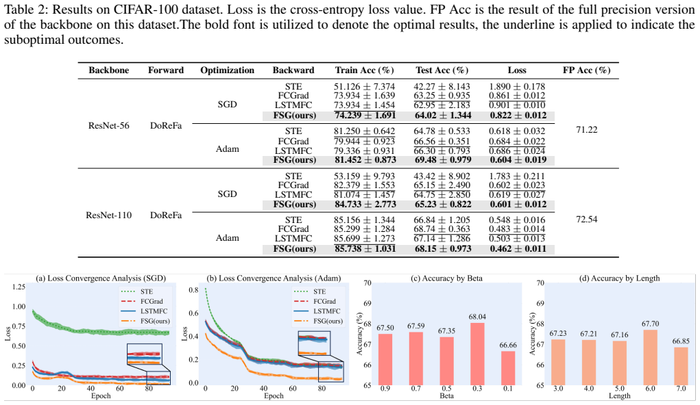
- The reported loss curves imply the learned momentum term helps most early in training, so FSG reaches a given loss in fewer epochs than STE, FCGrad, and LSTMFC.
- The extra training cost is confined to training: adding the slow-net raises per-epoch time by about 3.2 times in the overhead measurement, while at inference the binary network runs without either hypernetwork.
- Under the paper's convexity assumptions, the update rule is proved to converge at $O(1/\sqrt{t+1})$, matching the standard stochastic-subgradient rate, so the practical gains are claimed to come from better constants and better descent directions, not from an improved worst-case rate.
Reading between the lines
- The authors explicitly scope the experiments to ResNet-style convolutional networks; a direct next test is whether the same HGS and slow-net construction transfers to Transformer or LLM quantization, where gradient mismatch also appears.
- The reported optimum of $\beta=0.3$ implies the fast current-gradient branch should dominate; a sharper test would sweep $\beta$ jointly with history length $l$ and optimizer choice, since the paper fixes one hyperparameter at a time on a single dataset.
- Because the slow-net is shared across layers and only distinguished by a learned embedding, one could test whether the learned embeddings encode meaningful layer structure, for example by clustering the embeddings and comparing the clusters to layer depth.
Signed reviews
Editorial analysis
A structured set of objections, weighed in public.
Referee Report
Summary. The paper proposes FSG (Fast and Slow Gradient Generation), a hypernetwork-based method for training binary neural networks. It introduces a Historical Gradient Storage (HGS) module that keeps the last l flattened per-layer gradients, a slow-net (Mamba or LSTM) that consumes this history to produce a momentum-like gradient, a fast-net (MLP) that produces a current-gradient term, and Layer Recognition Embeddings (LRE) to make the shared slow-net layer-aware. The update rule is W^{t+1}_i = W^t_i - α M_f(g^t_{W_i}, \hat W^t_i) + β M_s(h^t_i). The authors report experiments on CIFAR-10 and CIFAR-100 with ResNet backbones, claiming faster convergence and lower loss than STE, FCGrad, LSTMFC, IR-Net, RBNN, and ReSTE, and include a convergence theorem with an appendix proof.
Significance. If the empirical claims are reliable, FSG would be a practical learned-gradient alternative to hand-designed straight-through estimators for BNNs, and the use of a sequence model over historical gradients is a reasonable idea worth exploring. The paper also makes a useful conceptual distinction between fast current-gradient generation and slow momentum generation, and it includes an ablation on the choice of slow-net and on the hyperparameters β and l. However, the significance is currently bounded by weaknesses in the evidence: duplicated baseline entries, a mislabeled overhead table, absent significance testing, and hyperparameter selection on the same benchmark used for the final comparison. The theoretical result is a conditional consistency statement rather than a convergence guarantee for the actual BNN training problem. These issues must be resolved before the central 'outperforms existing baselines' claim can be accepted.
major comments (5)
- [Table 1 and Table 2] The baseline entries contain implausible duplications. In Table 1, FCGrad and LSTMFC report exactly the same test accuracies on ResNet-32 and ResNet-44 under SGD (89.93 and 90.40, respectively), and in Table 2, FCGrad and LSTMFC report identical train accuracy (73.934) on ResNet-56 under SGD. Independent runs on different backbones would not produce identical values to three decimal places. This strongly suggests that rows were copied or mislabeled, and it undermines the reliability of the baseline numbers against which FSG is compared. The authors should provide the original run logs or correct the table entries and confirm that all baselines were measured under the same protocol.
- [Table 4] The headline CIFAR-100 comparison is not statistically supported. FSG reports 69.48 ± 0.979 while IR-Net reports 68.94 ± 0.967, a difference of 0.54 percentage points that is well within one standard deviation. The paper does not report paired significance tests, and the Reproducibility Checklist explicitly answers 'no' to the question about appropriate statistical tests. Without significance testing or a larger number of runs, the claim that FSG 'outperforms existing baselines' on CIFAR-100 is not established.
- [Ablation Experiment (Influence of β and l)] The hyperparameters β = 0.3 and l = 6 are selected on CIFAR-100 (Fig. 2c and 2d) and then reused for the CIFAR-100 comparison in Table 4. This means the reported CIFAR-100 margin over IR-Net is inflated by selection on the same benchmark used for the final evaluation. The authors should either report the selection procedure explicitly, evaluate on a held-out configuration, or correct for multiple testing. At minimum, they should state that the SOTA table configuration was chosen on the evaluation dataset.
- [Theorem 1 and Appendix proof] The convergence theorem assumes E_k[ M_s(ℏ_k) - (x_k - x_{k-1}) ] = 0, i.e., that the slow-net momentum equals the true momentum in expectation. This is precisely the desired behavior of the learned slow-net, so the theorem is a consistency result conditional on the slow-net being correct, not a guarantee that FSG converges for the BNN training objective. In addition, the assumptions of convex f_i, bounded iterates, and a bounded positive square-matrix fast-net do not match the nonconvex, binarized setting of the experiments. The theorem should be reframed as a conditional consistency property and the mismatch with the experimental setting should be acknowledged.
- [Table 5] The computational overhead table labels a row 'ReSTE' with Fast-net 'Multi MLP', Slow-net 'Mamba', and test accuracy 69.48. This does not match ReSTE, which is a rectified straight-through estimator rather than a hypernetwork-based method, and the reported 69.48 is the accuracy attributed to FSG elsewhere in the paper. The row appears mislabeled and the overhead comparison is therefore invalid. The authors should correct the row labels and clarify which method each runtime corresponds to.
minor comments (5)
- [Abstract and code URL] The Abstract states the code is available at github.com/FSG, while the text at the end of the Abstract and the introduction give http://github.com/two-tiger/FSG. This is inconsistent and the shorter URL appears to be a placeholder.
- [Equations (8) and (10)] The historical gradient index is inconsistent: Eq. (8) uses h^t_i = Concat[g^{t-l+1}_{w_i}, ..., g^t_{w_i}], while Eq. (10) writes the input as [t_i; g^{t-l}_{w_i} W_a, ..., g^t_{w_i} W_a]. The two equations describe different historical windows; please align them.
- [Equation (12) and Algorithm 1] Eq. (12) writes the forward update as A(W^t_i - α M_f(...) ∂A/∂W + β M_s(ℏ^t_i)), while Algorithm 1 line 4 writes Q{A[ W^t_i - α M_f(...) ∂A/∂W + β M_s(ℏ^t)] }. The placement of the parentheses differs and it is unclear whether the quantization is applied before or after the A(·) preprocessing. Please make the formulas consistent.
- [Theorem 1 proof] The proof uses ϕ_f and ϕ_s without clearly defining them; in some lines ϕ_f appears to denote the fast-net output and in others a scalar factor or linear map. This makes the proof difficult to follow. Please introduce notation explicitly and ensure that every symbol is defined before use.
- [Table 3 vs Table 4] Table 3 reports ResNet-56 CIFAR-100 accuracy of 68.04 ± 0.948 for the Mamba slow-net, while Table 2 and Table 4 report 69.48 ± 0.979 for FSG on the same backbone and dataset. The paper does not explain the discrepancy; please clarify the configuration difference (e.g., β, l, or optimizer settings) or correct the table.
Circularity Check
Partial circularity: hypernetwork training uses its own generated gradient as the learning signal, and CIFAR-100 hyperparameters are selected on the same benchmark used for the headline comparison; the broader empirical claim remains externally tested.
-
self definitional
[Training of FSG, Eqs. (12)-(14)]
"we register the generated gradient GF SG = βMs(ℏt i) − αMf (Gt Wi , ˆW t i ) ∂A(W t i ) ∂W t i in the optimizer to replace gW = ∂ℓ ∂W ... ∂ℓ ∂ϕt+1 f = ∂ℓ ∂ ˆW t+1 ∂ ˆW t+1 ∂ϕt+1 f = −α · GF SG ∂Mf (Gt Wi , ˆW t i ) ∂ϕt+1 f"
Equation (14) substitutes G_FSG for the true loss-gradient factor ∂ℓ/∂Ŵ^{t+1}, but G_FSG is itself defined as βM_s(ℏ^t) − αM_f(G_t,Ŵ_t)∂A/∂W, i.e. a function of the two hypernetworks being trained. The parameter updates for M_f and M_s therefore carry no independent loss-gradient information: the signal used to learn the generated gradient is the generated gradient itself. The paper's assertion that 'Mf and Ms are associated with the final loss' is not a derivation from the loss; it is a self-referential fixed-point loop, unless a separate true-loss term is silently used.
-
fitted input called prediction
[Ablation Experiment ('Influence of β', 'Influence of l'); applied in Table 4 (CIFAR-100)]
"Influence of β. In this experiments, we explore the sensitivity of the FSG method to the combination parameter β, selecting values of 0.9, 0.7, 0.5, 0.3, and 0.1 for evaluation on the CIFAR-100 dataset... the highest accuracy is achieved when β is set to 0.3. Influence of l. For l, we select 3, 4, 5, 6, and 7 to conduct experiments on CIFAR-100... the highest accuracy is achieved when l is set to 6."
The hyperparameters β and l are selected on the CIFAR-100 benchmark by directly maximizing accuracy, and the same CIFAR-100 accuracy (69.48 in Table 4) is then reported as evidence that FSG 'outperforms' IR-Net by 0.54%. The final CIFAR-100 comparison is therefore not an independent prediction: the reported margin is the objective used to pick the hyperparameters. This is a mild fitted-input-called-prediction form of circularity, confined to the CIFAR-100 SOTA claim rather than to the CIFAR-10 results.
full rationale
Most of the paper's contribution is empirical: FSG is tested against external baselines (DoReFa, IR-Net, RBNN, ReSTE, etc.) on CIFAR-10/100, so the headline 'outperforms' claim is not circular by construction. No load-bearing self-citation chain or imported uniqueness theorem is present; Mamba is chosen by ablation rather than by an authorial ansatz smuggled through a citation. Two genuine circular elements remain. First, the hypernetwork training loop in Eqs. (12)-(14) uses G_FSG, which is composed of the hypernetworks' own outputs, as the effective gradient for updating those hypernetworks; the asserted connection to the final loss is thus not an anchored loss-gradient signal but a self-consistency loop. Second, the CIFAR-100 SOTA comparison is weakened because β and l were tuned on CIFAR-100 and the same CIFAR-100 numbers are presented as the outperformance evidence. The convergence theorem is conditional on the explicit assumption E[M_s(h_k) − (x_k − x_{k−1})] = 0, which essentially postulates that the slow-net already produces the exact momentum; this is a strong, unproven premise rather than a formal circularity, since it is stated as an assumption. Overall, partial circularity in the training mechanism and in the CIFAR-100 evaluation, while the broader empirical method retains independent content.
Assumptions & free parameters
free parameters (6)
- beta =
0.3
- alpha =
0.3
- l (historical gradient memory length) =
6
- hidden dimension for fast-net and Mamba block expansion =
100
- hypernetwork learning rate =
1e-3 (Adam)
- backbone initial learning rate =
1e-3 CIFAR-10, 1e-1 CIFAR-100
assumptions (5)
- domain assumption The derivative of the sign/quantization function can be replaced by a learned surrogate generated by a hypernetwork without breaking gradient descent.
- domain assumption Momentum as a linear combination of historical gradients benefits optimization, so learning a momentum-like term from historical gradients benefits BNN training.
- ad hoc to paper A shared Mamba block can model flattened gradient sequences from different layers and filter noise, and a layer embedding suffices to disambiguate layers.
- ad hoc to paper In Theorem 1, the objective is convex, the stochastic gradient is unbiased with bounded variance, iterates stay bounded, the fast-net is a bounded positive square matrix, and the slow-net momentum error has zero expectation.
- domain assumption A well-trained full precision base model is available as initialization.
invented entities (4)
-
Historical Gradient Storage (HGS)
-
Fast-net MLP
-
Slow-net Mamba
-
Layer Recognition Embedding (LRE)
Cite this review
Pith. "Pith review of Fast and Slow Gradient Approximation for Binary Neural Network Optimization." pith.science (2026). https://pith.science/paper/6PRZCWM6
@misc{pith2026241211777,
  author       = {Pith},
  title        = {Pith review of: Fast and Slow Gradient Approximation for Binary Neural Network Optimization},
  year         = {2026},
  howpublished = {\url{https://pith.science/paper/6PRZCWM6}},
  note         = {Machine review of arXiv:2412.11777}
}
read the original abstract
Binary Neural Networks (BNNs) have garnered significant attention due to their immense potential for deployment on edge devices. However, the non-differentiability of the quantization function poses a challenge for the optimization of BNNs, as its derivative cannot be backpropagated. To address this issue, hypernetwork based methods, which utilize neural networks to learn the gradients of non-differentiable quantization functions, have emerged as a promising approach due to their adaptive learning capabilities to reduce estimation errors. However, existing hypernetwork based methods typically rely solely on current gradient information, neglecting the influence of historical gradients. This oversight can lead to accumulated gradient errors when calculating gradient momentum during optimization. To incorporate historical gradient information, we design a Historical Gradient Storage (HGS) module, which models the historical gradient sequence to generate the first-order momentum required for optimization. To further enhance gradient generation in hypernetworks, we propose a Fast and Slow Gradient Generation (FSG) method. Additionally, to produce more precise gradients, we introduce Layer Recognition Embeddings (LRE) into the hypernetwork, facilitating the generation of layer-specific fine gradients. Extensive comparative experiments on the CIFAR-10 and CIFAR-100 datasets demonstrate that our method achieves faster convergence and lower loss values, outperforming existing baselines.Code is available at http://github.com/two-tiger/FSG .
Figures

Reference graph
Works this paper leans on
-
[1]
, " * write output.state after.block = add.period write newline
ENTRY address archivePrefix author booktitle chapter edition editor eid eprint howpublished institution isbn journal key month note number organization pages publisher school series title type volume year label extra.label sort.label short.list INTEGERS output.state before.all mid.sentence after.sentence after.block FUNCTION init.state.consts #0 'before.a...
-
[2]
write newline
" write newline "" before.all 'output.state := FUNCTION n.dashify 't := "" t empty not t #1 #1 substring "-" = t #1 #2 substring "--" = not "--" * t #2 global.max substring 't := t #1 #1 substring "-" = "-" * t #2 global.max substring 't := while if t #1 #1 substring * t #2 global.max substring 't := if while FUNCTION word.in bbl.in capitalize " " * FUNCT...
-
[3]
Ajanthan, T.; Gupta, K.; Torr, P.; Hartley, R.; and Dokania, P. 2021. Mirror descent view for neural network quantization. In International conference on artificial intelligence and statistics, 2809--2817. PMLR
work page 2021
-
[4]
W.; Pfau, D.; Schaul, T.; Shillingford, B.; and De Freitas, N
Andrychowicz, M.; Denil, M.; Gomez, S.; Hoffman, M. W.; Pfau, D.; Schaul, T.; Shillingford, B.; and De Freitas, N. 2016. Learning to learn by gradient descent by gradient descent. Advances in neural information processing systems, 29
2016
-
[5]
Banner, R.; Hubara, I.; Hoffer, E.; and Soudry, D. 2018. Scalable methods for 8-bit training of neural networks. Advances in neural information processing systems, 31
work page 2018
-
[6]
Chen, H.; Wang, Y.; Xu, C.; Shi, B.; Xu, C.; Tian, Q.; and Xu, C. 2020. AdderNet: Do we really need multiplications in deep learning? In Proceedings of the IEEE/CVF conference on computer vision and pattern recognition, 1468--1477
work page 2020
-
[7]
Chen, S.; Wang, W.; and Pan, S. J. 2019. Metaquant: Learning to quantize by learning to penetrate non-differentiable quantization. Advances in Neural Information Processing Systems, 32
work page 2019
-
[8]
Courbariaux, M.; Bengio, Y.; and David, J.-P. 2015. Binaryconnect: Training deep neural networks with binary weights during propagations. Advances in neural information processing systems, 28
2015
Show all 32 references
-
[9]
Courbariaux, M.; Hubara, I.; Soudry, D.; El-Yaniv, R.; and Bengio, Y. 2016. Binarized neural networks: Training deep neural networks with weights and activations constrained to+ 1 or-1. arXiv preprint arXiv:1602.02830
2016 arXiv
-
[10]
L.; Zaremba, W.; Bruna, J.; LeCun, Y.; and Fergus, R
Denton, E. L.; Zaremba, W.; Bruna, J.; LeCun, Y.; and Fergus, R. 2014. Exploiting linear structure within convolutional networks for efficient evaluation. Advances in neural information processing systems, 27
2014
-
[11]
Devlin, J.; Chang, M.-W.; Lee, K.; and Toutanova, K. 2018. Bert: Pre-training of deep bidirectional transformers for language understanding. arXiv preprint arXiv:1810.04805
2018 arXiv
-
[12]
Ding, X.; Hao, T.; Tan, J.; Liu, J.; Han, J.; Guo, Y.; and Ding, G. 2021. Resrep: Lossless cnn pruning via decoupling remembering and forgetting. In Proceedings of the IEEE/CVF international conference on computer vision, 4510--4520
2021
-
[13]
A.; Van Gool, L.; Williams, C
Everingham, M.; Eslami, S. A.; Van Gool, L.; Williams, C. K.; Winn, J.; and Zisserman, A. 2015. The pascal visual object classes challenge: A retrospective. International journal of computer vision, 111: 98--136
2015
-
[14]
Girshick, R.; Donahue, J.; Darrell, T.; and Malik, J. 2014. Rich feature hierarchies for accurate object detection and semantic segmentation. In Proceedings of the IEEE conference on computer vision and pattern recognition, 580--587
2014
-
[15]
Gu, A.; and Dao, T. 2023. Mamba: Linear-Time Sequence Modeling with Selective State Spaces. arXiv preprint arXiv:2312.00752
2023 arXiv
-
[16]
Gu, A.; Goel, K.; and R\'e, C. 2022. Efficiently Modeling Long Sequences with Structured State Spaces. In The International Conference on Learning Representations ( ICLR )
2022
-
[17]
Hayashi, K.; Yamaguchi, T.; Sugawara, Y.; and Maeda, S.-i. 2019. Exploring unexplored tensor network decompositions for convolutional neural networks. Advances in Neural Information Processing Systems, 32
2019
-
[18]
He, K.; Zhang, X.; Ren, S.; and Sun, J. 2016. Deep residual learning for image recognition. In Proceedings of the IEEE conference on computer vision and pattern recognition, 770--778
2016
-
[19]
Hochreiter, S.; and Schmidhuber, J. 1997. Long Short-Term Memory. Neural Computation, 9(8): 1735--1780
1997
-
[20]
N.; Han, S.; Moskewicz, M
Iandola, F. N.; Han, S.; Moskewicz, M. W.; Ashraf, K.; Dally, W. J.; and Keutzer, K. 2016. SqueezeNet: AlexNet-level accuracy with 50x fewer parameters and< 0.5 MB model size. arXiv preprint arXiv:1602.07360
2016 arXiv
-
[21]
Krizhevsky, A.; Hinton, G.; et al. 2009. Learning multiple layers of features from tiny images
2009
-
[22]
LeCun, Y.; Bengio, Y.; and Hinton, G. 2015. Deep learning. nature, 521(7553): 436--444
2015
-
[23]
Lin, M.; Ji, R.; Xu, Z.; Zhang, B.; Wang, Y.; Wu, Y.; Huang, F.; and Lin, C.-W. 2020. Rotated binary neural network. Advances in neural information processing systems, 33: 7474--7485
2020
-
[24]
Liu, J.; Wen, D.; Wang, D.; Tao, W.; Chen, T.-W.; Osa, K.; and Kato, M. 2020. QuantNet: Learning to quantize by learning within fully differentiable framework. In Computer Vision--ECCV 2020 Workshops: Glasgow, UK, August 23--28, 2020, Proceedings, Part V 16, 38--53. Springer
2020
-
[25]
Luo, J.-H.; Wu, J.; and Lin, W. 2017. Thinet: A filter level pruning method for deep neural network compression. In Proceedings of the IEEE international conference on computer vision, 5058--5066
2017
-
[26]
Qin, H.; Gong, R.; Liu, X.; Shen, M.; Wei, Z.; Yu, F.; and Song, J. 2020. Forward and backward information retention for accurate binary neural networks. In Proceedings of the IEEE/CVF conference on computer vision and pattern recognition, 2250--2259
2020
-
[27]
Rastegari, M.; Ordonez, V.; Redmon, J.; and Farhadi, A. 2016. Xnor-net: Imagenet classification using binary convolutional neural networks. In European conference on computer vision, 525--542. Springer
2016
-
[28]
Saad, D. 1998. Online algorithms and stochastic approximations. Online Learning, 5(3): 6
1998
-
[29]
Wu, X.-M.; Zheng, D.; Liu, Z.; and Zheng, W.-S. 2023. Estimator meets equilibrium perspective: A rectified straight through estimator for binary neural networks training. In Proceedings of the IEEE/CVF International Conference on Computer Vision, 17055--17064
2023
-
[30]
Xu, Y.; Han, K.; Xu, C.; Tang, Y.; Xu, C.; and Wang, Y. 2021. Learning frequency domain approximation for binary neural networks. Advances in Neural Information Processing Systems, 34: 25553--25565
2021
-
[31]
Zhou, S.; Wu, Y.; Ni, Z.; Zhou, X.; Wen, H.; and Zou, Y. 2016. Dorefa-net: Training low bitwidth convolutional neural networks with low bitwidth gradients. arXiv preprint arXiv:1606.06160
2016 arXiv
-
[32]
Zhu, L.; Liao, B.; Zhang, Q.; Wang, X.; Liu, W.; and Wang, X. 2024. Vision Mamba: Efficient Visual Representation Learning with Bidirectional State Space Model. arXiv preprint arXiv:2401.09417
2024 arXiv
Reviewed August 11, 2026 · model on record in the stance chip above.
Discussion (0). Continue with ORCID to comment.