REVIEW 3 major objections 5 minor 88 references
Scalable Temporal Anomaly Causality Discovery in Large Systems: Achieving Computational Efficiency with Binary Anomaly Flag Data
T0 review · 3 major / 5 minor · reviewed 2026-08-11 · deepseek-v4-flash
Pith's one-line read The paper claims that temporal causal graphs can be learned from sparse binary anomaly flags by compressing uniform regions, excluding self-lag and non-overlapping links, and testing only anomaly-triggering positive associations.
desk verdict Solid computational-efficiency result for causal discovery on sparse binary flags, but the accuracy comparison is likely biased by treating PCMCI's self-loops as false positives. read the letter →
The pith
A machine-rendered reading of the paper's core claim, the machinery that carries it, and where it could break.
The reading
What carries the argument
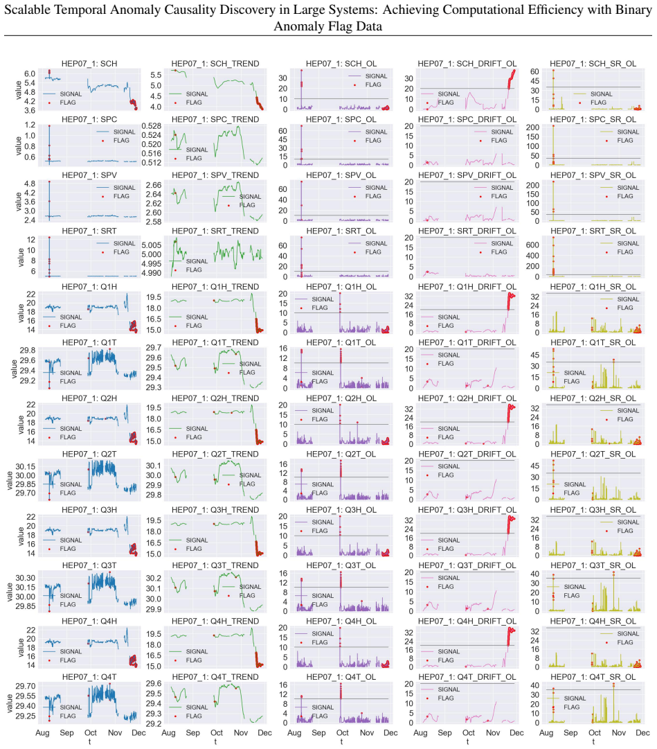
The load-bearing mechanism is the sparse-data handler in Algorithm 2: it detects stretches where every sensor's anomaly flag is unchanged (all 0 or all 1), keeps only the first $l_m$ samples of each stretch, with $l_m$ set slightly larger than the causal search horizon $\tau_{\max}$, and discards the rest. This shrinks the Hadron Calorimeter stream from roughly 400K to about 900 samples and the public IT stream by 55%. Around this sit three further mechanisms: the prior-link assumption that drops self-lag edges and non-overlapping links, reducing the PCMCI conditional-independence load from $O(n'(N\tau_{\max})^2)$ to $O(n'\sum_i N_i' \tau_{\max}^2)$; the anomaly-aware CI test (ANAC), which uses partial correlation on residuals and keeps only positive associations so that causality is read from 0 to 1 flag transitions rather than from lingering one-runs; and a pruning step that keeps the strongest or earliest lag for cyclic links and orients residual undirected edges with a chi-square test so the final object is a DAG suitable for Bayesian-network inference.
What would settle it
Generate a synthetic binary time series from a known graph in which each sensor's flag at time $t$ depends on its own flag at $t-1$ and on one cross-sensor cause, then run AnomalyCD with self-lags excluded; if the learned graph contains spurious cross-sensor edges that are absent from the generating DAG, the self-lag exclusion is the cause and the central accuracy claim does not transfer to self-persistent alarm streams.
Extended reading notes
Core claim
The paper claims that causal structure can be recovered from binary anomaly flags by treating flag transitions, not raw associations, as the signal, and by aggressively compressing long runs of unchanged flags. AnomalyCD combines an anomaly-aware conditional independence test called ANAC, which uses partial correlation on residuals and keeps only positive associations corresponding to anomaly occurrence; a sparse data handler that compresses uniform 0/0 or 1/1 regions while preserving a short prefix of each region so time-lag structure survives; a prior-link assumption that excludes self-lag edges and non-overlapping edges, cutting the PCMCI link-search space; and a post-processing pruning step that removes cyclic and bidirected edges and orients remaining undirected edges with a chi-square test. On the public IT dataset the full pipeline improves F1 over plain PCMCI from 0.302 to 0.364, and with directed edge orientation precision rises from 0.182 to 0.333. On the Hadron Calorimeter data, the learned graph links temperature anomalies to Peltier regulator responses in a way that matches the physical circuit.
Load-bearing premise
The framework assumes that a sensor's own past anomaly flag is not a cause of its current flag and that only temporally overlapping sensor flags can be causally related; if flag persistence is self-generated, the graph may misattribute that persistence to other sensors.
Editorial extensions
If this is right
- Operators can run graph learning on alarm streams that were previously too large: the Hadron Calorimeter stream's roughly 400K samples compress to about 900, and PCMCI skeleton learning completes in under 19 seconds on a laptop-class CPU.
- Root-cause queries become quantitative: the Bayesian network built on the pruned graph computes conditional anomaly probabilities, such as $P(\text{Q1T}=1 \mid \text{Q2T}=1)$ rising from 0.05 to 0.90 at lag zero, giving operators ranked suspects.
- The compression step is a general preprocessing layer: most of the 12 comparison methods improve on compressed data, with an average relative F1 gain of 18.31% when two underperforming methods are excluded, so compressed binary flags help other causal learners, not only AnomalyCD.
- Anomaly-induced graphs can differ from normal-operation graphs: on the public IT dataset AnomalyCD ranks near the top among the compared methods even though the scoring reference graph describes normal operation, not the anomaly regime.
Reading between the lines
- Beyond the paper, the self-lag exclusion deserves a direct test: because anomaly flags persist by construction, a sensor's own past flag is a strong predictor of its current flag, and removing that edge may push explained variance onto overlapping sensors; a synthetic experiment with known self-causal flags would isolate this effect.
- Beyond the paper, the 99.76% compression suggests event-based causal discovery, which treats 0-to-1 transitions as point events, as a complementary route; AnomalyCD keeps a short prefix of uniform regions, but a point-process formulation could drop the prefix altogether and reduce the data even further.
- Beyond the paper, the accuracy numbers on the public dataset may understate real performance: the reference graph describes normal operation, while anomaly-induced graphs can differ, so a larger fraction of the recovered edges may be true anomaly-specific causality than the F1 reflects.
Editorial analysis
A structured set of objections, weighed in public.
Referee Report
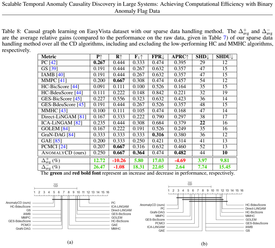
Summary. The paper proposes AnomalyCD, a pipeline for temporal causal discovery on binary anomaly-flag time series. It combines an online univariate anomaly detector, sparse-data compression that retains only the first lm samples of each uniform flag region, a PCMCI-based graph learner using a positive-partial-correlation CI test (ANAC), a prior-link handler that excludes self-lag and non-overlapping edges, and post-hoc pruning of multi-lag and bidirected edges. The method is evaluated on HCAL readout-box sensor data and on the public EasyVista IT monitoring dataset. The authors report that compression reduces the HCAL data by 99.76% and the EasyVista data by 55%, lowers PCMCI skeleton runtime from about 34.6 s at lm=30 to 19.0 s at lm=10, and improves F1 on EasyVista from 0.302 (PCMCI) to 0.364 (AnomalyCD). The central claims are considerable computational savings and a moderate accuracy improvement for causal discovery from binary anomaly flags.
Significance. If the accuracy comparison is made fair, this would be a useful practical contribution to root-cause analysis on alarm-flag data: the compression idea is simple, the runtime measurements are concrete, the EasyVista comparison covers 16 baseline methods, and the authors provide code. The computational-efficiency claim is well supported. However, the accuracy claim is currently entangled with a modeling assumption that excludes self-lag causality, and the HCAL accuracy table has missing entries at the main operating point. Because the accuracy improvement is the weaker and less established half of the contribution, the paper should be revised before the accuracy claim is accepted.
major comments (3)
- [§4.2.2 (Algorithm 3), §5.2 (Table 9, Figure 14)] The reported F1 gain over PCMCI is confounded by the prior link assumption that excludes self-lag causality. The EasyVista reference graph in Figure 14 is a summary graph with no self-loops, whereas the PCMCI baseline can output lagged self-dependencies; after temporal-to-summary aggregation, those self-loops count as false positives. AnomalyCD's change relative to PCMCI (precision 0.182 to 0.250, recall 0.889 to 0.667) is exactly the pattern expected from deleting self-loops. The ablation in Table 9 never scores a variant that keeps self-lags and removes them symmetrically from both outputs, so the reader cannot tell how much of the 0.302 to 0.364 F1 gain is a scoring artifact. Since binary anomaly flags are persistent by construction, excluding self-lags can also attribute a variable's own persistence to other sensors and create spurious cross-sensor edges. Please add an experiment in which self-loops are treated symmetrically in all methods, or the reference graph includes self-loops, so the accuracy gain can be evaluated independently of this assumption.
- [§5.1.2, Table 4] The HCAL experiment does not support the accuracy half of the computational-accuracy tradeoff at the main operating point. Table 4 reports APRC and SHD for lm=10, the setting used for the 99.76% compression claim, as dashes, and it does not state what reference graph the APRC and SHD scores are computed against. Without a specified reference, these scores only measure agreement among the algorithm's own outputs at different compression lengths. Please specify the reference graph and provide the missing lm=10 accuracy values, or explicitly limit the HCAL claim to computational savings plus qualitative graph plausibility.
- [§3.2, §5.2] The accuracy evaluation uses a normal-operation causal graph (Figure 14) as the reference, while the method learns an anomaly-regime graph from binary flags whose anomalies are all collective with the same appearance time and duration (Section 3.2). The authors acknowledge this mismatch in the discussion, but it still weakens the accuracy claim: agreement with a normal-operation graph is not the same as accuracy on the anomaly-regime graph. A synthetic experiment with known ground-truth anomaly-regime edges, persistence, and lags would substantially strengthen the claim; without it, the accuracy improvement should be described as agreement with a normal-operation reference rather than as causal graph accuracy per se.
minor comments (5)
- [Title and running header] The running header contains the typo 'A CHIEVING'; the title should read 'Achieving Computational Efficiency'.
- [§2.3, Eq. (4)] The text says the joint distribution is the sum of all CPDs in the network, but Eq. (4) is a product; please correct the wording.
- [Table 3 and Algorithm 3] The symbol ατ is used for the trend-drift threshold in Table 3 and for the overlap-strength threshold in Algorithm 3; please use distinct symbols to avoid confusion.
- [Algorithm 2] The function name 'CompressBinayData' should be 'CompressBinaryData'.
- [Eq. (12)] The SHD definition is informal; please define the binary adjacency matrices G and H explicitly so that N(i,j) is a clear count of mismatched edges.
Circularity Check
No circular derivation: accuracy claims rest on external benchmark; self-citations are inputs, and the self-lag exclusion is an explicit prior, not a fitted prediction.
full rationale
The paper's central accuracy claim is benchmarked externally on the EasyVista dataset against 16 baselines with a reference graph from Assaad et al., so it is not derived from the authors' own prior results. The components credited for the gain (ANAC, sparse data compression, edge pruning) are algorithmic transformations with stated assumptions, not fitted parameters renamed as predictions. The heavy self-citations (refs. 13-16, 62) supply trained anomaly-detection models and the RBX selection; these are inputs to the framework, not evidence used to conclude that the framework works. The prior-link assumption in Section 4.2.2, which 'excludes self-lag causality and non-overlapping links,' is an explicit modeling and computational choice; whether it inflates precision in the summary-graph evaluation against PCMCI by removing self-loop false positives is a benchmark-fairness and correctness concern, not circularity, because the prior is not fitted to the reference graph and the comparison is externally anchored. The paper also candidly states limitations, including BN bidirectional edges indicating confounding, the reference graph being derived from normal operations, and hyperparameter tuning effort. No predicted quantity reduces to an input by construction; score 2 reflects the presence of non-load-bearing self-citation rather than any actual circular step.
Assumptions & free parameters
free parameters (5)
- anomaly detection thresholds (alpha_theta, alpha_tau, alpha_eta) =
10, 20, 35 for HCAL; alpha_eta=2 for EasyVista
- sparse compression length lm =
10
- maximum time-lag tau_max =
5
- CI test significance pv =
0.05
- overlap strength threshold alpha_tau (Algorithm 3) =
not specified
assumptions (5)
- domain assumption Causal Markov condition and faithfulness hold for the alarm-flag variables
- domain assumption Causal sufficiency: no unobserved common causes of the monitored sensors
- ad hoc to paper Positive partial correlation between anomaly flags is necessary and sufficient for causation
- ad hoc to paper A sensor's own past flag and non-overlapping flags cannot be causes
- ad hoc to paper Uniform flag regions carry no causal information beyond their first lm samples
Cite this review
Pith. "Pith review of Scalable Temporal Anomaly Causality Discovery in Large Systems: Achieving Computational Efficiency with Binary Anomaly Flag Data." pith.science (2026). https://pith.science/paper/QGUIDZXQ
@misc{pith2026241211800,
  author       = {Pith},
  title        = {Pith review of: Scalable Temporal Anomaly Causality Discovery in Large Systems: Achieving Computational Efficiency with Binary Anomaly Flag Data},
  year         = {2026},
  howpublished = {\url{https://pith.science/paper/QGUIDZXQ}},
  note         = {Machine review of arXiv:2412.11800}
}
read the original abstract
Extracting anomaly causality facilitates diagnostics once monitoring systems detect system faults. Identifying anomaly causes in large systems involves investigating a broader set of monitoring variables across multiple subsystems. However, learning graphical causal models (GCMs) comes with a significant computational burden that restrains the applicability of most existing methods in real-time and large-scale deployments. In addition, modern monitoring applications for large systems often generate large amounts of binary alarm flags, and the distinct characteristics of binary anomaly data -- the meaning of state transition and data sparsity -- challenge existing causality learning mechanisms. This study proposes an anomaly causal discovery approach (AnomalyCD), addressing the accuracy and computational challenges of generating GCMs from temporal binary flag datasets. The AnomalyCD presents several strategies, such as anomaly data-aware causality testing, sparse data and prior link compression, and edge pruning adjustment approaches. We validate the performance of the approach on two datasets: monitoring sensor data from the readout-box system of the Compact Muon Solenoid experiment at CERN, and a public dataset from an information technology monitoring system. The results on temporal GCMs demonstrate a considerable reduction of computation overhead and a moderate enhancement of accuracy on the binary anomaly datasets. Code: https://github.com/muleina/AnomalyCD .
Figures


Figures from the paper (14 more)





Reference graph
Works this paper leans on
-
[1]
Data-driven root-cause fault diagnosis for multivariate non-linear processes,
B. Rashidi, D. S. Singh, and Q. Zhao, “Data-driven root-cause fault diagnosis for multivariate non-linear processes,”Control Engineering Practice, vol. 70, pp. 134–147, 2018
2018
-
[2]
PEN: process estimator neural network for root cause analysis using graph convolution,
V . Leonhardt, F. Claus, and C. Garth, “PEN: process estimator neural network for root cause analysis using graph convolution,” Journal of Manufacturing Systems, vol. 62, pp. 886–902, 2022. 24 Scalable Temporal Anomaly Causality Discovery in Large Systems: Achieving Computational Efficiency with Binary Anomaly Flag Data
2022
-
[3]
High-recall causal discovery for autocorrelated time series with latent confounders,
A. Gerhardus and J. Runge, “High-recall causal discovery for autocorrelated time series with latent confounders,” Advances in Neural Information Processing Systems, vol. 33, pp. 12 615–12 625, 2020
2020
-
[4]
FLAGS: a methodology for adaptive anomaly detection and root cause analysis on sensor data streams by fusing expert knowledge with machine learning,
B. Steenwinckel, D. De Paepe, S. V . Hautte, P. Heyvaert, M. Bentefrit, P. Moens, A. Dimou, B. Van Den Bossche, F. De Turck, S. Van Hoecke et al., “FLAGS: a methodology for adaptive anomaly detection and root cause analysis on sensor data streams by fusing expert knowledge with machine learning,” Future Generation Computer Systems, vol. 116, pp. 30–48, 2021
2021
-
[5]
Root cause analysis in the industrial domain using knowledge graphs: a case study on power transformers,
J. Martinez-Gil, G. Buchgeher, D. Gabauer, B. Freudenthaler, D. Filipiak, and A. Fensel, “Root cause analysis in the industrial domain using knowledge graphs: a case study on power transformers,” Procedia Computer Science, vol. 200, pp. 944–953, 2022
2022
-
[6]
Review of causal discovery methods based on graphical models,
C. Glymour, K. Zhang, and P. Spirtes, “Review of causal discovery methods based on graphical models,”Frontiers in genetics, vol. 10, p. 524, 2019
2019
-
[7]
A survey of learning causality with data: problems and methods,
R. Guo, L. Cheng, J. Li, P. R. Hahn, and H. Liu, “A survey of learning causality with data: problems and methods,” ACM Computing Surveys, vol. 53, no. 4, pp. 1–37, 2020
2020
-
[8]
Root-cause analysis for time-series anomalies via spatiotemporal graphical modeling in distributed complex systems,
C. Liu, K. G. Lore, Z. Jiang, and S. Sarkar, “Root-cause analysis for time-series anomalies via spatiotemporal graphical modeling in distributed complex systems,” Knowledge-Based Systems, vol. 211, p. 106527, 2021
2021
Show all 88 references
-
[9]
Mining association rules for anomaly detection in dynamic process runtime behavior and explaining the root cause to users,
K. Böhmer and S. Rinderle-Ma, “Mining association rules for anomaly detection in dynamic process runtime behavior and explaining the root cause to users,” Information Systems, vol. 90, p. 101438, 2020
2020
-
[10]
Causal network construction based on convergent cross mapping (ccm) for alarm system root cause tracing of nonlinear industrial process,
C. Tian, C. Zhao, H. Fan, and Z. Zhang, “Causal network construction based on convergent cross mapping (ccm) for alarm system root cause tracing of nonlinear industrial process,” IFAC-PapersOnLine, vol. 53, no. 2, pp. 13 619–13 624, 2020
2020
-
[11]
Causal discovery with attention-based convolutional neural networks,
M. Nauta, D. Bucur, and C. Seifert, “Causal discovery with attention-based convolutional neural networks,”Machine Learning and Knowledge Extraction, vol. 1, no. 1, pp. 312–340, 2019
2019
-
[12]
Root cause diagnosis in multivariate time series based on modified temporal convolution and multi-head self-attention,
Y . Zhou, K. Xu, and F. He, “Root cause diagnosis in multivariate time series based on modified temporal convolution and multi-head self-attention,” Journal of Process Control, vol. 117, pp. 14–25, 2022
2022
-
[13]
Unsupervised deep variational model for multivariate sensor anomaly detection,
M. W. Asres, G. Cummings, P. Parygin, A. Khukhunaishvili, M. Toms, A. Campbell, S. I. Cooper, D. Yu, J. Dittmann, and C. W. Omlin, “Unsupervised deep variational model for multivariate sensor anomaly detection,” inInternational Conference on Progress in Informatics and Computi...
2021
-
[14]
Long horizon anomaly prediction in multivariate time series with causal autoencoders,
M. W. Asres, G. Cummings, A. Khukhunaishvili, P. Parygin, S. I. Cooper, D. Yu, J. Dittmann, and C. W. Omlin, “Long horizon anomaly prediction in multivariate time series with causal autoencoders,” in PHM Society European Conference, vol. 7, no. 1, 2022, pp. 21–31
2022
-
[15]
Spatio-temporal anomaly detection with graph networks for data quality monitoring of the Hadron Calorimeter,
M. W. Asres, C. W. Omlin, L. Wang, D. Yu, P. Parygin, J. Dittmann, G. Karapostoli, M. Seidel, R. Venditti, L. Lambrechtet al., “Spatio-temporal anomaly detection with graph networks for data quality monitoring of the Hadron Calorimeter,” Sensors, vol. 23, no. 24, p. 9679, 2023
2023
-
[16]
Data quality monitoring through transfer learning on anomaly detection for the Hadron Calorimeters,
M. W. Asres, C. W. Omlin, L. Wang, P. Parygin, D. Yu, J. Dittmann, and The CMS-HCAL Collaboration, “Data quality monitoring through transfer learning on anomaly detection for the Hadron Calorimeters,” arXiv preprint arXiv:2408.16612, 2024
2024
-
[17]
Anomaly detection using deep autoencoders for the assessment of the quality of the data acquired by the CMS experiment,
A. A. Pol, V . Azzolini, G. Cerminara, F. De Guio, G. Franzoni, M. Pierini, F. Sirok`y, and J.-R. Vlimant, “Anomaly detection using deep autoencoders for the assessment of the quality of the data acquired by the CMS experiment,” in European Physical Journal Web of Conferences,...
2019
-
[18]
The model of an anomaly detector for HiLumi LHC magnets based on recurrent neural networks and adaptive quantization,
M. Wielgosz, M. Mertik, A. Skocze ´n, and E. De Matteis, “The model of an anomaly detector for HiLumi LHC magnets based on recurrent neural networks and adaptive quantization,” Engineering Applications of Artificial Intelligence, vol. 74, pp. 166–185, 2018
2018
-
[19]
Autoencoder-based anomaly detection system for online data quality monitoring of the cms electromagnetic calorimeter,
D. Abadjiev, “Autoencoder-based anomaly detection system for online data quality monitoring of the cms electromagnetic calorimeter,” Fermi National Accelerator Laboratory (FNAL), Batavia, IL (United States), Tech. Rep., 2023
2023
-
[20]
Framework for inferring empirical causal graphs from binary data to support multidimensional poverty analysis,
C. Amornbunchornvej, N. Surasvadi, A. Plangprasopchok, and S. Thajchayapong, “Framework for inferring empirical causal graphs from binary data to support multidimensional poverty analysis,” Heliyon, vol. 9, no. 5, 2023
2023
-
[21]
Causal structure-based root cause analysis of outliers,
K. Budhathoki, L. Minorics, P. Blöbaum, and D. Janzing, “Causal structure-based root cause analysis of outliers,” inInterna- tional Conference on Machine Learning. Proceedings of Machine Learning Research, 2022, pp. 2357–2369
2022
-
[22]
Causal network reconstruction from time series: from theoretical assumptions to practical estimation,
J. Runge, “Causal network reconstruction from time series: from theoretical assumptions to practical estimation,” Chaos: an Interdisciplinary Journal of Nonlinear Science, vol. 28, no. 7, 2018
2018
-
[23]
Detecting and quantifying causal associations in large nonlinear time series datasets,
J. Runge, P. Nowack, M. Kretschmer, S. Flaxman, and D. Sejdinovic, “Detecting and quantifying causal associations in large nonlinear time series datasets,” Science Advances, vol. 5, no. 11, p. eaau4996, 2019
2019
-
[24]
Discovering contemporaneous and lagged causal relations in autocorrelated nonlinear time series datasets,
J. Runge, “Discovering contemporaneous and lagged causal relations in autocorrelated nonlinear time series datasets,” in Conference on Uncertainty in Artificial Intelligence. Proceedings of Machine Learning Research, 2020, pp. 1388–1397
2020
-
[25]
Reconstructing regime-dependent causal relationships from observa- tional time series,
E. Saggioro, J. de Wiljes, M. Kretschmer, and J. Runge, “Reconstructing regime-dependent causal relationships from observa- tional time series,” Chaos: an Interdisciplinary Journal of Nonlinear Science, vol. 30, no. 11, 2020
2020
-
[26]
R. E. Neapolitan et al., Learning Bayesian networks. Pearson Prentice Hall, 2004, vol. 38. 25 Scalable Temporal Anomaly Causality Discovery in Large Systems: Achieving Computational Efficiency with Binary Anomaly Flag Data
2004
-
[27]
CloudRanger: root cause identification for cloud native systems,
P. Wang, J. Xu, M. Ma, W. Lin, D. Pan, Y . Wang, and P. Chen, “CloudRanger: root cause identification for cloud native systems,” in 18th International Symposium on Cluster, Cloud and Grid Computing. IEEE, 2018, pp. 492–502
2018
-
[28]
Localizing failure root causes in a microservice through causality inference,
Y . Meng, S. Zhang, Y . Sun, R. Zhang, Z. Hu, Y . Zhang, C. Jia, Z. Wang, and D. Pei, “Localizing failure root causes in a microservice through causality inference,” in 28th International Symposium on Quality of Service. IEEE, 2020, pp. 1–10
2020
-
[29]
Spirtes, C
P. Spirtes, C. N. Glymour, and R. Scheines, Causation, prediction, and search. MIT press, 2000
2000
-
[30]
CausalBench: a large-scale benchmark for network inference from single-cell perturbation data,
M. Chevalley, Y . Roohani, A. Mehrjou, J. Leskovec, and P. Schwab, “CausalBench: a large-scale benchmark for network inference from single-cell perturbation data,” arXiv preprint arXiv:2210.17283, 2022
2022 arXiv
-
[31]
Root cause identification for collective anomalies in time series given an acyclic summary causal graph with loops,
C. K. Assaad, I. Ez-Zejjari, and L. Zan, “Root cause identification for collective anomalies in time series given an acyclic summary causal graph with loops,” in International Conference on Artificial Intelligence and Statistics . Proceedings of Machine Learning Research, 2023...
2023
-
[32]
Multi-lag and multi-type temporal causality inference and analysis for industrial process fault diagnosis,
J. Chen and C. Zhao, “Multi-lag and multi-type temporal causality inference and analysis for industrial process fault diagnosis,” Control Engineering Practice, vol. 124, p. 105174, 2022
2022
-
[33]
Detection and root cause analysis of multiple plant-wide oscillations using multivariate nonlinear chirp mode decomposition and multivariate Granger causality,
Q. Chen, X. Lang, S. Lu, N. ur Rehman, L. Xie, and H. Su, “Detection and root cause analysis of multiple plant-wide oscillations using multivariate nonlinear chirp mode decomposition and multivariate Granger causality,” Computers and Chemical Engineering, vol. 147, p. 107231, 2021
2021
-
[34]
Root cause analysis of industrial faults based on binary extreme gradient boosting and temporal causal discovery network,
K. Qin, L. Chen, J. Shi, Z. Li, and K. Hao, “Root cause analysis of industrial faults based on binary extreme gradient boosting and temporal causal discovery network,” Chemometrics and Intelligent Laboratory Systems, vol. 225, p. 104559, 2022
2022
-
[35]
Fault detection and diagnosis using bayesian network model combining mechanism correlation analysis and process data: application to unmonitored root cause variables type faults,
N. Liu, M. Hu, J. Wang, Y . Ren, and W. Tian, “Fault detection and diagnosis using bayesian network model combining mechanism correlation analysis and process data: application to unmonitored root cause variables type faults,” Process Safety and Environmental Protection, vol. ...
2022
-
[36]
A generalized matrix profile framework with support for contextual series analysis,
D. De Paepe, S. V . Hautte, B. Steenwinckel, F. De Turck, F. Ongenae, O. Janssens, and S. Van Hoecke, “A generalized matrix profile framework with support for contextual series analysis,”Engineering Applications of Artificial Intelligence, vol. 90, p. 103487, 2020
2020
-
[37]
Why did the distribution change?
K. Budhathoki, D. Janzing, P. Bloebaum, and H. Ng, “Why did the distribution change?” in International Conference on Artificial Intelligence and Statistics. Proceedings of Machine Learning Research, 2021, pp. 1666–1674
2021
-
[38]
A unified approach to interpreting model predictions,
S. M. Lundberg and S.-I. Lee, “A unified approach to interpreting model predictions,” in Advances in Neural Information Processing Systems. Curran Associates, Inc., 2017, vol. 30, pp. 4765–4774
2017
-
[39]
Learning bayesian network model structure from data,
D. Margaritis et al., “Learning bayesian network model structure from data,” Ph.D. dissertation, School of Computer Science, Carnegie Mellon University Pittsburgh, PA, USA, 2003
2003
-
[40]
Algorithms for large scale Markov blanket discovery,
I. Tsamardinos, C. F. Aliferis, A. R. Statnikov, and E. Statnikov, “Algorithms for large scale Markov blanket discovery,” in FLAIRS conference, vol. 2. St. Augustine, FL, 2003, pp. 376–380
2003
-
[41]
Time and sample efficient discovery of Markov blankets and direct causal relations,
I. Tsamardinos, C. F. Aliferis, and A. Statnikov, “Time and sample efficient discovery of Markov blankets and direct causal relations,” in Proceedings of the 9th ACM SIGKDD International Conference on Knowledge Discovery and Data Mining, 2003, pp. 673–678
2003
-
[42]
Order-independent constraint-based causal structure learning,
D. Colombo, M. H. Maathuis et al., “Order-independent constraint-based causal structure learning,” Journal of Machine Learning Research, vol. 15, no. 1, pp. 3741–3782, 2014
2014
-
[43]
The max-min hill-climbing bayesian network structure learning algorithm,
I. Tsamardinos, L. E. Brown, and C. F. Aliferis, “The max-min hill-climbing bayesian network structure learning algorithm,” Machine Learning, vol. 65, pp. 31–78, 2006
2006
-
[44]
Koller and N
D. Koller and N. Friedman, Probabilistic graphical models: principles and techniques. MIT press, 2009
2009
-
[45]
Optimal structure identification with greedy search,
D. M. Chickering, “Optimal structure identification with greedy search,” Journal of machine learning research, vol. 3, no. Nov, pp. 507–554, 2002
2002
-
[46]
Scaling up greedy causal search for continuous variables,
J. D. Ramsey, “Scaling up greedy causal search for continuous variables,” arXiv preprint arXiv:1507.07749, 2015
2015 arXiv
-
[47]
A hybrid causal search algorithm for latent variable models,
J. M. Ogarrio, P. Spirtes, and J. Ramsey, “A hybrid causal search algorithm for latent variable models,” in Conference on Probabilistic Graphical Models. Proceedings of Machine Learning Research, 2016, pp. 368–379
2016
-
[48]
CAM: causal additive models, high-dimensional order search and penalized regression,
P. Bühlmann, J. Peters, and J. Ernest, “CAM: causal additive models, high-dimensional order search and penalized regression,” The Annals of Statistics, vol. 42, pp. 2526–2556, 2014
2014
-
[49]
Learning functional causal models with generative neural networks,
O. Goudet, D. Kalainathan, P. Caillou, I. Guyon, D. Lopez-Paz, and M. Sebag, “Learning functional causal models with generative neural networks,” Explainable and Interpretable Models in Computer Vision and Machine Learning, pp. 39–80, 2018
2018
-
[50]
Peters, D
J. Peters, D. Janzing, and B. Schölkopf, Elements of causal inference: foundations and learning algorithms. The MIT Press, 2017
2017
-
[51]
Simplified granger causality map for data-driven root cause diagnosis of process disturbances,
Y . Liu, H.-S. Chen, H. Wu, Y . Dai, Y . Yao, and Z. Yan, “Simplified granger causality map for data-driven root cause diagnosis of process disturbances,” Journal of Process Control, vol. 95, pp. 45–54, 2020
2020
-
[52]
Granger causality: a review and recent advances,
A. Shojaie and E. B. Fox, “Granger causality: a review and recent advances,” Annual Review of Statistics and Its Application, vol. 9, pp. 289–319, 2022. 26 Scalable Temporal Anomaly Causality Discovery in Large Systems: Achieving Computational Efficiency with Binary Anomaly Flag Data
2022
-
[53]
Statistical perspective on functional and causal neural connectomics: the time-aware pc algorithm,
R. Biswas and E. Shlizerman, “Statistical perspective on functional and causal neural connectomics: the time-aware pc algorithm,” PLOS Computational Biology, vol. 18, no. 11, p. e1010653, 2022
2022
-
[54]
Investigating causal relations by econometric models and cross-spectral methods,
C. W. Granger, “Investigating causal relations by econometric models and cross-spectral methods,”Econometrica: Journal of the Econometric Society, pp. 424–438, 1969
1969
-
[55]
Neural Granger causality,
A. Tank, I. Covert, N. Foti, A. Shojaie, and E. B. Fox, “Neural Granger causality,”IEEE Transactions on Pattern Analysis and Machine Intelligence, vol. 44, no. 8, pp. 4267–4279, 2021
2021
-
[56]
The CMS experiment at the CERN LHC,
The CMS Collaboration, S. Chatrchyan, G. Hmayakyan, V . Khachatryan, A. Sirunyan, W. Adam, T. Bauer, T. Bergauer, H. Bergauer, M. Dragicevic et al., “The CMS experiment at the CERN LHC,” Journal of Instrumentation, vol. 3, p. S08004, 2008
2008
-
[57]
Development of the CMS detector for the CERN LHC Run 3,
A. Hayrapetyan et al., “Development of the CMS detector for the CERN LHC Run 3,” JINST, vol. 19, no. 05, p. P05064, 2024
2024
-
[58]
The upgrade of the CMS Hadron Calorimeter with Silicon photomultipliers,
N. Strobbe, “The upgrade of the CMS Hadron Calorimeter with Silicon photomultipliers,” Journal of Instrumentation, vol. 12, no. 1, p. C01080, 2017
2017
-
[59]
Status of the CMS detector,
E. Focardi, “Status of the CMS detector,” Physics Procedia, vol. 37, pp. 119–127, 2012
2012
-
[60]
CMS technical design report for the phase 1 upgrade of the hadron calorimeter,
J. Mans, “CMS technical design report for the phase 1 upgrade of the hadron calorimeter,” CMS-TDR-010, Tech. Rep., 2012
2012
-
[61]
Design, performance, and calibration of CMS Hadron Endcap calorimeters,
G. Baiatian, M. Hashemi, S. Hagopian, A. Pal, E. Machado, E. Isiksal, V . ODell, T. Haelen, D. A. Sanders, E. Yazganet al., “Design, performance, and calibration of CMS Hadron Endcap calorimeters,” CERN-CMS-NOTE-2008-010, Tech. Rep., 2008
2008
-
[62]
Lightweight multi- system multivariate interconnection and divergence discovery,
M. W. Asres, C. W. Omlin, J. Dittmann, P. Parygin, J. Hiltbrand, S. I. Cooper, G. Cummings, and D. Yu, “Lightweight multi- system multivariate interconnection and divergence discovery,” in19th Annual System of Systems Engineering Conference (SoSE), 2024
2024
-
[63]
EasyVista,
“EasyVista,” https://www.easyvista.com/fr/produits/ev-observe, accessed: 2023-01-10
2023
-
[64]
EasyRCA IT monitoring dataset,
“EasyRCA IT monitoring dataset,” https://github.com/ckassaad/EasyRCA, accessed: 2023-01-10
2023
-
[65]
Multivariate LSTM-FCNs for time series classification,
F. Karim, S. Majumdar, H. Darabi, and S. Harford, “Multivariate LSTM-FCNs for time series classification,”Neural Networks, vol. 116, pp. 237–245, 2019
2019
-
[66]
STL: a seasonal-trend decomposition,
R. B. Cleveland, W. S. Cleveland, J. E. McRae, and I. Terpenning, “STL: a seasonal-trend decomposition,”J. Off. Stat, vol. 6, no. 1, pp. 3–73, 1990
1990
-
[67]
A fully automated periodicity detection in time series,
T. Puech, M. Boussard, A. D’Amato, and G. Millerand, “A fully automated periodicity detection in time series,” inAdvanced Analytics and Learning on Temporal Data: 4th ECML PKDD Workshop. Springer, 2020, pp. 43–54
2020
-
[68]
ClaSP: parameter-free time series segmentation,
A. Ermshaus, P. Schäfer, and U. Leser, “ClaSP: parameter-free time series segmentation,” Data Mining and Knowledge Discovery, vol. 37, no. 3, pp. 1262–1300, 2023
2023
-
[69]
MSTL: a seasonal-trend decomposition algorithm for time series with multiple seasonal patterns,
K. Bandara, R. J. Hyndman, and C. Bergmeir, “MSTL: a seasonal-trend decomposition algorithm for time series with multiple seasonal patterns,” arXiv preprint arXiv:2107.13462, 2021
2021 arXiv
-
[70]
Time-series anomaly detection service at Microsoft,
H. Ren, B. Xu, Y . Wang, C. Yi, C. Huang, X. Kou, T. Xing, M. Yang, J. Tong, and Q. Zhang, “Time-series anomaly detection service at Microsoft,” in Proceedings of the 25th ACM SIGKDD International Conference on Knowledge Discovery and Data Mining, 2019, pp. 3009–3017
2019
-
[71]
Comprehensive review and empirical evaluation of causal discovery algorithms for numerical data,
W. Niu, Z. Gao, L. Song, and L. Li, “Comprehensive review and empirical evaluation of causal discovery algorithms for numerical data,” arXiv preprint arXiv:2407.13054, 2024
2024 arXiv
-
[72]
Enhancing causal discovery from robot sensor data in dynamic scenarios,
L. Castri, S. Mghames, M. Hanheide, and N. Bellotto, “Enhancing causal discovery from robot sensor data in dynamic scenarios,” in Conference on Causal Learning and Reasoning. PMLR, 2023, pp. 243–258
2023
-
[73]
Y . M. Bishop, S. E. Fienberg, and P. W. Holland,Discrete multivariate analysis: theory and practice. Springer Science and Business Media, 2007
2007
-
[74]
K. P. Murphy,Dynamic Bayesian networks: representation, inference and learning. University of California, Berkeley, 2002
2002
-
[75]
A novel dynamic Bayesian network approach for data mining and survival data analysis,
A. Sheidaei, A. R. Foroushani, K. Gohari, and H. Zeraati, “A novel dynamic Bayesian network approach for data mining and survival data analysis,” BMC Medical Informatics and Decision Making, vol. 22, no. 1, pp. 1–15, 2022
2022
-
[76]
Optimal detection of changepoints with a linear computational cost,
R. Killick, P. Fearnhead, and I. A. Eckley, “Optimal detection of changepoints with a linear computational cost,”Journal of the American Statistical Association, vol. 107, no. 500, pp. 1590–1598, 2012
2012
-
[77]
New efficient algorithms for multiple change-point detection with reproducing kernels,
A. Celisse, G. Marot, M. Pierre-Jean, and G. Rigaill, “New efficient algorithms for multiple change-point detection with reproducing kernels,” Computational Statistics and Data Analysis, vol. 128, pp. 200–220, 2018
2018
-
[78]
Structural intervention distance for evaluating causal graphs,
J. Peters and P. Bühlmann, “Structural intervention distance for evaluating causal graphs,”Neural Computation, vol. 27, no. 3, pp. 771–799, 2015
2015
-
[79]
gcastle: a python toolbox for causal discovery,
K. Zhang, S. Zhu, M. Kalander, I. Ng, J. Ye, Z. Chen, and L. Pan, “gcastle: a python toolbox for causal discovery,” arXiv preprint arXiv:2111.15155, 2021
2021 arXiv
-
[80]
Scoring functions for learning bayesian networks,
A. M. Carvalho, “Scoring functions for learning bayesian networks,” Inesc-id Tec. Rep, vol. 12, pp. 1–48, 2009
2009
-
[81]
Di- rectLiNGAM: a direct method for learning a linear non-Gaussian structural equation model,
S. Shimizu, T. Inazumi, Y . Sogawa, A. Hyvarinen, Y . Kawahara, T. Washio, P. O. Hoyer, K. Bollen, and P. Hoyer, “Di- rectLiNGAM: a direct method for learning a linear non-Gaussian structural equation model,”Journal of Machine Learning Research, vol. 12, no. Apr, pp. 1225–1248...
2011
-
[82]
A linear non-Gaussian acyclic model for causal discovery,
S. Shimizu, P. O. Hoyer, A. Hyvärinen, A. Kerminen, and M. Jordan, “A linear non-Gaussian acyclic model for causal discovery,” Journal of Machine Learning Research, vol. 7, no. 10, 2006
2006
-
[83]
Gradient-based neural dag learning,
S. Lachapelle, P. Brouillard, T. Deleu, and S. Lacoste-Julien, “Gradient-based neural dag learning,” arXiv preprint arXiv:1906.02226, 2019
1906 arXiv
-
[84]
On the role of sparsity and dag constraints for learning linear dags,
I. Ng, A. Ghassami, and K. Zhang, “On the role of sparsity and dag constraints for learning linear dags,” Advances in Neural Information Processing Systems, vol. 33, pp. 17 943–17 954, 2020
2020
-
[85]
A graph autoencoder approach to causal structure learning,
I. Ng, S. Zhu, Z. Chen, and Z. Fang, “A graph autoencoder approach to causal structure learning,” arXiv preprint arXiv:1911.07420, 2019
1911 arXiv
-
[86]
Causal discovery with reinforcement learning,
S. Zhu, I. Ng, and Z. Chen, “Causal discovery with reinforcement learning,” arXiv preprint arXiv:1906.04477, 2019
1906 arXiv
-
[87]
Ordering-based causal discovery with reinforcement learning,
X. Wang, Y . Du, S. Zhu, L. Ke, Z. Chen, J. Hao, and J. Wang, “Ordering-based causal discovery with reinforcement learning,” arXiv preprint arXiv:2105.06631, 2021
2021 arXiv
-
[88]
P. B. Nemenyi, Distribution-free multiple comparisons. Princeton University, 1963. 28 The CMS-HCAL Collaboration M.W. Asres 1, C.W. Omlin 1, V . Chekhovsky2,a, A. Chinaryan 2, A. Gevorgyan 2, Ya. Halkin 2, A. Kunts 2, A. Litomin 2,a, A. Petrosyan2, A. Tumasyan 2, H. Saka 3, A....
1963
Reviewed August 11, 2026 · model on record in the stance chip above.
Discussion (0). Continue with ORCID to comment.