REVIEW 3 major objections 6 minor 35 references
PowerMLP: An Efficient Version of KAN
T0 review · 3 major / 6 minor · reviewed 2026-08-11 · deepseek-v4-flash
Pith's one-line read PowerMLP, an MLP-style network using k-th powers of ReLU as activations, is claimed to match KAN's function space on bounded boxes while training roughly 40 times faster.
desk verdict Useful empirical speedup and a clean architecture, but the central same-depth equivalence with KAN is false; worth a careful revision, not acceptance as-is. read the letter →
The pith
A machine-rendered reading of the paper's core claim, the machinery that carries it, and where it could break.
The reading
What carries the argument
The load-bearing identity is Lemma 1: a $k$-order B-spline on a knot sequence $(t_j,\dots,t_{j+k+1})$ equals $\sum_i \frac{t_{j+k+1}-t_j}{\prod_{l\neq i}(t_l-t_i)}\,\sigma_k(x-t_i)$. This expresses the recursive de Boor-Cox construction as a single fixed linear combination of ReLU powers, which is what lets PowerMLP evaluate splines without iteration; the same identity is inverted in Lemmas 4 and 5 to show splines can also reproduce affine maps and ReLU-$k$, giving the reverse inclusion over bounded intervals.
What would settle it
Train a one-hidden-layer KAN with a $(3,3)$-grid and compare the functions it can express with a one-hidden-layer PowerMLP of width $w^2(G+k)$: if there exists a KAN function that no same-depth PowerMLP of that width reproduces, the inclusion in Theorem 2 fails as stated. Concretely, check whether the $\beta$ matrix in Eq. (11) can always be absorbed into the following layer without changing the number of layers, since removing that absorption step breaks the depth equality in the theorem.
Extended reading notes
Core claim
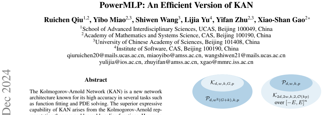
The paper's central discovery is that KAN's learnable spline activations are redundant in a precise sense: every $(k,G)$-spline is a linear combination of $k$-th powers of ReLU, so any KAN layer can be rewritten as a PowerMLP layer with the same number of trainable parameters and a width inflated by a factor of $G+k$. This yields the inclusion $K_{d,w,k,G,p} \subset P_{d,w^2(G+k),k,p}$, and since splines vanish outside their support while ReLU powers generate all polynomials, PowerMLPs form a strictly larger function space over $\mathbb{R}^n$. Conversely, over any bounded interval, affine maps and ReLU-$k$ functions can be represented by splines, so every PowerMLP layer is a two-layer KAN; the two architectures therefore define the same function space on $[-E,E]^n$. The paper also derives closed-form FLOP counts showing KAN needs over ten times more operations per parameter, and validates the theory with experiments reporting roughly 40-fold faster training.
Load-bearing premise
The proof of Theorem 2 rewrites a KAN layer as $\beta\sigma_k(\omega x+\gamma)$ and then assumes the post-activation matrix $\beta$ can be folded into the next layer without changing the depth count, but the PowerMLP layer as defined has no such post-activation linear map, so the same-depth inclusion depends on a depth re-counting that the definition does not state.
Editorial extensions
If this is right
- Any architecture that uses KAN layers can swap in PowerMLP layers and keep, or exceed, the representable function space while cutting training time by roughly 40x in the reported settings.
- The approximation guarantee for smooth functions on $[-1,1]^n$ (Corollary 8) transfers to KANs via the equivalence on bounded intervals, giving a depth and parameter bound for KANs that goes beyond the depth-2 Kolmogorov-Arnold representation.
- PowerMLP has FLOP counts close to plain MLP, so MLP-optimized hardware and training pipelines can be reused without the spline-evaluation overhead.
- The ablation indicates the basis function is needed for training stability at depth and ReLU-$k$ for expressive power, so both components are load-bearing in practice.
Reading between the lines
- Beyond the paper: if the equivalence on bounded intervals holds, then approximation and representation results for ReLU-$k$ MLPs transfer to KANs and vice versa, a two-way bridge the paper only sketches through Corollary 8.
- Beyond the paper: the FLOP comparison counts forward-pass arithmetic only; a fairer training-cost comparison would include backward passes and memory access, so the reported 40x wall-clock speedup may depend on implementation details beyond FLOPs.
- Beyond the paper: the strictly-larger-over-$\mathbb{R}^n$ claim suggests that MLP-type networks need not sacrifice expressive power to gain speed, which could inform architecture search beyond KAN itself.
Editorial analysis
A structured set of objections, weighed in public.
Referee Report
Summary. The paper proposes PowerMLP, a feedforward network whose hidden layers compute αℓ b(xℓ) + σ_k(ωℓ xℓ + γℓ) and whose last layer is affine, as a faster MLP-style alternative to Kolmogorov-Arnold Networks. The theoretical sections claim that B-splines can be written as linear combinations of powers of ReLU, that any KAN is contained in a PowerMLP of the same depth and comparable width (Theorem 2), and that the reverse inclusion holds over bounded intervals using a two-layer KAN construction (Theorem 6), yielding an equality of function spaces (Corollary 7) and an approximation bound (Corollary 8). The paper also provides a FLOPs comparison and experiments on function fitting, knot theory, classification, and training time, reporting training speeds about 40 times faster than KAN.
Significance. The practical motivation is credible: a drop-in network that trains much faster than KAN while retaining comparable accuracy would be useful, and the empirical study is substantial: the experiments use matched parameter budgets, repeated timings, ablations, and released code. The reverse inclusion PowerMLP ⊆ KAN over intervals (Theorem 6) appears to be a valid construction. However, the central theoretical contribution is not established. The key inclusion Theorem 2 is false as stated, and Corollary 3 and Corollary 7 both depend on it. As a result, the advertised claims that PowerMLPs define a strictly larger or equal function space than KANs are unsupported. The empirical speed and accuracy results may still be of interest, but they do not compensate for the failure of the main theoretical assertion in a paper whose abstract, title, and Figure 1 foreground that assertion.
major comments (3)
- [Section 4.2 / Definition 3 (Eq. 6), Eq. 11] The proof of Theorem 2 does not establish the stated inclusion K_{d,w,k,G,p} ⊂ P_{d,w^2(G+k),k,p}. The proof models a KAN layer as αb(x) + βσ_k(ωx + γ) in Eq. (11), but Definition 3 (Eq. (6)) contains no post-activation matrix β: the only term added after σ_k is αb(x), where α multiplies the fixed basis function b(x), not the activated features. The assertion that β can be absorbed into the next layer is not a reparameterization of the same network, because the next PowerMLP layer applies σ_k to an affine function of its input, so the absorbed β would enter inside the next nonlinearity, whereas in the KAN the multiplication by β occurs before the next layer's spline activation. For the final layer there is no next layer, and Eq. (6) makes the final PowerMLP layer affine. Consequently, a depth-1 KAN whose single layer is a nonlinear spline (e.g., a (3,3)-spline representing x^2 on [-1,1]) cannot be represented by any depth-1 PowerMLP. The same-depth inclusion is therefore false as stated, and Corollary 3 and Corollary 7, which both rely on Theorem 2, are not established.
- [Appendix A.1, parameter accounting] The proof's parameter accounting is inconsistent with the PowerMLP architecture. The proof introduces β ∈ R^{m×mn(G+k)} and counts mn(G+k) parameters for β, but those parameters do not appear in Definition 3. If β is instead absorbed into the following layer, that layer's weight matrix changes, so the claimed equality of parameter counts for a same-depth network is lost. Thus the subscript p in P_{d,w^2(G+k),k,p} is not supported by the proof.
- [Section 4.2, Corollary 3] Even setting aside the failure of Theorem 2, the argument for strict inclusion over R^n is incomplete. The text says that a spline function is zero outside a certain interval and that PowerMLPs include all polynomials, but a KAN layer also contains the residual basis function b(x) in Eq. (4), which is nonzero and unbounded outside that interval. To conclude that KANs cannot represent all polynomials, the paper would need to analyze the effect of composing b(x) with spline layers; this is not done. The strictness claim is therefore unsupported independently of the Theorem 2 gap.
minor comments (6)
- [Definition 3, Eq. (6)] The dimension of γℓ is stated as R^{mℓ×1}, but ωℓ is m_{ℓ+1}×mℓ, so ωℓ xℓ + γℓ lives in R^{m_{ℓ+1}×1}; the bias dimension should be corrected.
- [Eq. (11) and surrounding text] Eq. (11) writes βσ_{k-1}(ωx + γ) while the text and the rest of the proof use σ_k; this is presumably a typo and should be made consistent.
- [Lemma 1 proof] The proof uses σ_0(x) as the binary step function, but Eq. (5) defines σ_k only for k ∈ Z_+; σ_0 should be defined explicitly or the base case should be stated as a convention.
- [Section 5.3, Table 3] The reported speedup ratios vary from about 24× to 95× across the eight tasks; writing 'about 40 times faster' is only an average, and the range or standard deviation should be reported.
- [Section 5.2, Figure 5] The accuracy comparisons in Figure 5 appear as single points without error bars or repetition information; adding variability would strengthen the empirical claims.
- [Related Work / Section 5] The related work mentions KAN variants such as Wav-KAN and rKAN, but the experiments compare only against KAN version 0.2.5; a comparison with at least one faster KAN implementation would make the speed claim more robust.
Circularity Check
No circularity found; the theoretical derivation rests on external classical spline results and independent approximation theorems.
full rationale
The paper's central claims are not circular in the sense defined here. Lemma 1 (B-splines as linear combinations of powers of ReLU) is justified by the classical Curry-Schoenberg and Greville results, not by the paper's own conclusions. Theorem 2 is proven from Lemma 1 by explicitly constructing α, β, ω, γ; the later claim that β can be absorbed into the next layer is a mathematical gap in the depth accounting (and a correctness risk), but it is not a self-referential reduction of a prediction to a fitted input. Theorem 6 and Corollary 7 use external spline facts and de Boor's partition-of-unity property, and Corollary 8 imports the approximation bound from Li, Tang, and Yu (2020a), which is independent of this paper's fitted values. The FLOPs comparison follows Yu, Yu, and Wang (2024) for KAN arithmetic counts and does not fit parameters to outcomes. No fitted constant is renamed as a prediction, no load-bearing self-citation appears, and no uniqueness or representation theorem is imported from the authors' own prior work. The experimental speed and accuracy results are evaluated against external benchmarks and are not used to define the theoretical statements.
Assumptions & free parameters
assumptions (5)
- domain assumption KAN architecture with residual basis b(x)=x/(1+e^{-x}) and (k,G)-spline activations (Liu et al. 2024) is the baseline being compared.
- standard math B-splines with distinct knots can be represented as finite linear combinations of truncated power functions (Curry-Schoenberg 1947; Greville 1969).
- standard math B-spline partition of unity sum_j B_{j,k}(x)=1 on t0≤x≤tG (de Boor 1978).
- standard math RePU networks approximate functions f with ∫∑(∂f)^2≤1 at rate O(ε^{-n}) with O(n log^2 1/ε) layers (Li, Tang, Yu 2020a, Theorem 3.3).
- domain assumption Knot sequences used by KAN are increasing, hence distinct knots for Lemma 1.
Cite this review
Pith. "Pith review of PowerMLP: An Efficient Version of KAN." pith.science (2026). https://pith.science/paper/J3UVPDGW
@misc{pith2026241213571,
  author       = {Pith},
  title        = {Pith review of: PowerMLP: An Efficient Version of KAN},
  year         = {2026},
  howpublished = {\url{https://pith.science/paper/J3UVPDGW}},
  note         = {Machine review of arXiv:2412.13571}
}
read the original abstract
The Kolmogorov-Arnold Network (KAN) is a new network architecture known for its high accuracy in several tasks such as function fitting and PDE solving. The superior expressive capability of KAN arises from the Kolmogorov-Arnold representation theorem and learnable spline functions. However, the computation of spline functions involves multiple iterations, which renders KAN significantly slower than MLP, thereby increasing the cost associated with model training and deployment. The authors of KAN have also noted that ``the biggest bottleneck of KANs lies in its slow training. KANs are usually 10x slower than MLPs, given the same number of parameters.'' To address this issue, we propose a novel MLP-type neural network PowerMLP that employs simpler non-iterative spline function representation, offering approximately the same training time as MLP while theoretically demonstrating stronger expressive power than KAN. Furthermore, we compare the FLOPs of KAN and PowerMLP, quantifying the faster computation speed of PowerMLP. Our comprehensive experiments demonstrate that PowerMLP generally achieves higher accuracy and a training speed about 40 times faster than KAN in various tasks.
Figures


Figures from the paper (4 more)


Reference graph
Works this paper leans on
-
[1]
, " * write output.state after.block = add.period write newline
ENTRY address archivePrefix author booktitle chapter edition editor eid eprint howpublished institution isbn journal key month note number organization pages publisher school series title type volume year label extra.label sort.label short.list INTEGERS output.state before.all mid.sentence after.sentence after.block FUNCTION init.state.consts #0 'before.a...
-
[2]
write newline
" write newline "" before.all 'output.state := FUNCTION n.dashify 't := "" t empty not t #1 #1 substring "-" = t #1 #2 substring "--" = not "--" * t #2 global.max substring 't := t #1 #1 substring "-" = "-" * t #2 global.max substring 't := while if t #1 #1 substring * t #2 global.max substring 't := if while FUNCTION word.in bbl.in capitalize " " * FUNCT...
-
[3]
Aghaei, A. A. 2024. rKAN: Rational Kolmogorov-Arnold Networks. arXiv preprint arXiv:2406.14495
arXiv 2024
-
[4]
Becker, B.; and Kohavi, R. 1996. Adult . UCI Machine Learning Repository. DOI : https://doi.org/10.24432/ C5XW20
work page 1996
-
[5]
Bozorgasl, Z.; and Chen, H. 2024. Wav-KAN: Wavelet Kolmogorov-Arnold Networks. arXiv preprint arXiv:2405.12832
arXiv 2024
-
[6]
D.; Mastropietro, A.; Anagnostopoulos, A.; and Aris
Carlo, G. D.; Mastropietro, A.; Anagnostopoulos, A.; and Aris. 2024. Kolmogorov-Arnold Graph Neural Networks. arXiv preprint arXiv:2406.18354
arXiv 2024
-
[7]
Cox, M. G. 1972. The Numerical Evaluation of B-Splines . IMA Journal of Applied Mathematics, 10(2): 134--149
work page 1972
-
[8]
Curry, H. B.; and Schoenberg, I. J. 1947. On spline distributions and their limits-the polya distribution functions. Bulletin of the American Mathematical Society, 53(11): 1114--1114
work page 1947
Show all 35 references
-
[9]
Davies, A.; Juh \'a sz, A.; Lackenby, M.; and Tomasev, N. 2022. The signature and cusp geometry of hyperbolic knots. arXiv preprint arXiv:2111.15323
2022 arXiv
-
[10]
Davies, A.; Veli c kovi \'c , P.; Buesing, L.; Blackwell, S.; Zheng, D.; Toma s ev, N.; Tanburn, R.; Battaglia, P.; Blundell, C.; Juh \'a sz, A.; et al. 2021. Advancing mathematics by guiding human intuition with AI. Nature, 600(7887): 70--74
2021
-
[11]
de Boor, C. 1978. A Practical Guide to Splines, volume 27. New York: Springer
1978
-
[12]
Galitsky, B. A. 2024. Kolmogorov-Arnold network for word-level explainable meaning representation. Preprints
2024
-
[13]
Glorot, X.; Bordes, A.; and Bengio, Y. 2011. Deep Sparse Rectifier Neural Networks. In Proceedings of the Fourteenth International Conference on Artificial Intelligence and Statistics, volume 15 of Proceedings of Machine Learning Research, 315--323
2011
-
[14]
M.; Bringas, G
G \'o mez Hidalgo, J. M.; Bringas, G. C.; S \'a nz, E. P.; and Garc \' a, F. C. 2006. Content based SMS spam filtering. In Proceedings of the 2006 ACM symposium on Document engineering, 107--114
2006
-
[15]
Greville, T. 1969. Theory and Applications of Spline Functions. Army. Mathematics Research Center, Madison, Wis. Publication. Academic Press. ISBN 9780123029508
1969
-
[16]
Haykin, S. 1998. Neural Networks: A Comprehensive Foundation. USA: Prentice Hall PTR, 2nd edition. ISBN 0132733501
1998
-
[17]
He, K.; Zhang, X.; Ren, S.; and Sun, J. 2015. Delving deep into rectifiers: Surpassing human-level performance on imagenet classification. In Proceedings of the IEEE international conference on computer vision, 1026--1034
2015
-
[18]
Hendrycks, D.; and Gimpel, K. 2023. Gaussian Error Linear Units (GELUs). arXiv preprint arXiv:1606.08415
2023 arXiv
-
[19]
Inzirillo, H.; and Genet, R. 2024. SigKAN: Signature-Weighted Kolmogorov-Arnold Networks for Time Series. arXiv preprint arXiv:2406.17890
2024 arXiv
-
[20]
Kiamari, M.; Kiamari, M.; Kiamari, M.; and Krishnamachari, B. 2024. GKAN: Graph Kolmogorov-Arnold Networks. arXiv preprint arXiv:2406.06470
2024 arXiv
-
[21]
S.; Henderson, D.; Howard, R
LeCun, Y.; Boser, B.; Denker, J. S.; Henderson, D.; Howard, R. E.; Hubbard, W.; and Jackel, L. D. 1989. Backpropagation applied to handwritten zip code recognition. Neural computation, 1(4): 541--551
1989
-
[22]
LeCun, Y.; Bottou, L.; Bengio, Y.; and Haffner, P. 1998. Gradient-based learning applied to document recognition. Proceedings of the IEEE, 86(11): 2278--2324
1998
-
[23]
Li, B.; Tang, S.; and Yu, H. 2020 a . Better Approximations of High Dimensional Smooth Functions by Deep Neural Networks with Rectified Power Units. Communications in Computational Physics, 27(2): 379--411
2020
-
[24]
Li, B.; Tang, S.; and Yu, H. 2020 b . PowerNet: Efficient Representations of Polynomials and Smooth Functions by Deep Neural Networks with Rectified Power Units. J. Math. Study, 53(2): 159--191
2020
-
[25]
Li, Z. 2024. Kolmogorov-Arnold Networks are Radial Basis Function Networks. arXiv preprint arXiv:2405.06721
2024 arXiv
-
[26]
Y.; and Tegmark, M
Liu, Z.; Wang, Y.; Vaidya, S.; Ruehle, F.; Halverson, J.; Solja x i c , M.; Hou, T. Y.; and Tegmark, M. 2024. KAN: Kolmogorov-Arnold Networks. arXiv preprint arXiv:2404.19756v4
2024 arXiv
-
[27]
L.; Hannun, A
Maas, A. L.; Hannun, A. Y.; Ng, A. Y.; et al. 2013. Rectifier nonlinearities improve neural network acoustic models. In Proc. icml, volume 30, 3
2013
-
[28]
Mhaskar, H. N. 1993. Approximation properties of a multilayered feedforward artificial neural network. Advances in Computational Mathematics, 1: 61--80
1993
-
[29]
Molchanov, P.; Tyree, S.; Karras, T.; Aila, T.; and Kautz, J. 2017. Pruning Convolutional Neural Networks for Resource Efficient Inference. arXiv preprint arXiv:1611.06440
2017 arXiv
-
[30]
Y.; et al
Netzer, Y.; Wang, T.; Coates, A.; Bissacco, A.; Wu, B.; Ng, A. Y.; et al. 2011. Reading digits in natural images with unsupervised feature learning. In NIPS workshop on deep learning and unsupervised feature learning
2011
-
[31]
Ramos, J.; et al. 2003. Using tf-idf to determine word relevance in document queries. In Proceedings of the first instructional conference on machine learning, volume 242, 29--48
2003
-
[32]
Vaswani, A. 2017. Attention is all you need. arXiv preprint arXiv:1706.03762
2017 arXiv
-
[33]
Xu, K.; Chen, L.; and Wang, S. 2024. Kolmogorov-Arnold Networks for Time Series: Bridging Predictive Power and Interpretability. arXiv preprint arXiv:2406.02496
2024 arXiv
-
[34]
Yu, R.; Yu, W.; and Wang, X. 2024. KAN or MLP: A Fairer Comparison. arXiv preprint arXiv:2407.16674
2024 arXiv
-
[35]
Zhang, X.; Zhao, J.; and LeCun, Y. 2015. Character-level convolutional networks for text classification. Advances in neural information processing systems, 28
2015
Reviewed August 11, 2026 · model on record in the stance chip above.
Discussion (0). Continue with ORCID to comment.