Characterizations of sharp solute-solvent interfaces in hydrophobic environments via cylindrical coordinates

Hao Xiao

REVIEW 5 major objections 6 minor 41 references

Characterizations of sharp solute-solvent interfaces in hydrophobic environments via cylindrical coordinates

T0 review · 5 major / 6 minor · reviewed 2026-08-11 · deepseek-v4-flash

Challenge this review Re-run · record.json Download PDF Read on arXiv ↗ Review JSON

Pith's one-line read This paper shows that sharp solute-solvent interfaces around two hydrophobic Gay-Berne ellipsoids, including the hard-to-find saddle (transition) interface, can be computed as solutions of an ODE boundary value problem obtained from the…

desk verdict A plausible ODE reduction for symmetric two-ellipsoid VISM, but the saddle-interface claim is not yet supported as written. read the letter →

arxiv 2412.13590 v1 pith:QMDP55BZ submitted 2024-12-18 cond-mat.soft

Hao Xiao This is my paper · ORCID

classification cond-mat.soft MSC 35R3549Q1065L10

keywords solute-solventinterfacehydrophobicsolvationvariationalimplicitsolventmodelGay-BerneellipsoidssharpsaddleODEboundaryvalueproblemcylindricalcoordinates

verification ladder T0 review T1 audit T2 compute T3 formal

The pith

A machine-rendered reading of the paper's core claim, the machinery that carries it, and where it could break.

The reading

The paper establishes that for two identical hydrophobic Gay-Berne ellipsoidal molecules placed symmetrically about the origin, the sharp solute-solvent interface—both the stable minimum and the saddle transition state—is described by a second-order nonlinear ODE in cylindrical coordinates. This reduces the full three-dimensional free-energy minimization of the variational implicit solvent model to a boundary value problem that can be solved with a standard solver. The method reproduces connected stable, connected saddle, and disconnected stable interfaces for a molecule separation D=10 Å, and it tracks how the neck radius rmin changes with D. The significance is that saddle interfaces, which are the transition states for dewetting-driven hydrophobic collapse, were previously very hard to compute in implicit-solvent models.

What carries the argument

The central object is the cylindrical-coordinate parameterization of the interface as a surface of revolution, with r(z) for the inter-solute neck and z(r) for the end caps. The governing equation is the first variation of the VISM free energy, P + 2γ0[H - τK] = ρ0 U, where H is mean curvature, K is Gaussian curvature, τ is the Tolman length, and U is the Gay-Berne Lennard-Jones potential of the two ellipsoids. The key reduction uses the principal curvatures for a surface of revolution to convert this into the nonlinear ODE (3.1), and the saddle computation rescales the z-domain to s∈[0,1] with d as an unknown parameter (eq. 3.2), imposing r(0)=rmin and r'(1)=0. The disconnected portions are handled by two additional ODEs (3.4) and (3.5) with boundary conditions fixed by the neck's maximum radius.

What would settle it

Evaluate the free energy G on the computed saddle surface for D=10 Å and compute its second variation; if the surface is not a stationary point with exactly one negative eigenvalue, the imposed boundary conditions have selected a different solution family. Alternatively, solve the full 3D PDE (1.11) without the symmetry assumption for the same parameters and check that its saddle solution matches the ODE result.

Watch

Extended reading notes

Core claim

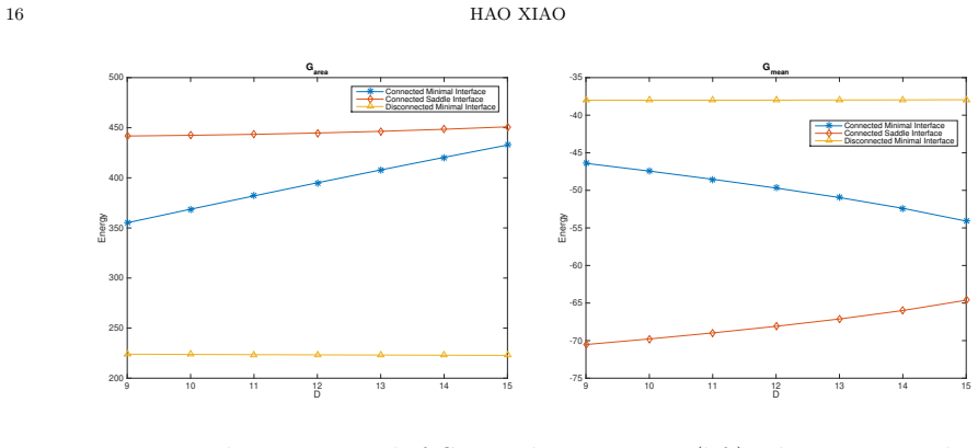
Within the variational implicit solvent model (VISM), the sharp solute-solvent interface is a surface of revolution r=r(z) (or z=z(r)) about the axis through the two Gay-Berne ellipsoid centers. Substituting the curvature formulas for a surface of revolution into the Euler-Lagrange equation P + 2γ0(H - τK) = ρ0 U turns the free-boundary PDE into the ODE (3.1) for the connected portion and (3.4)/(3.5) for the cap portions. The paper's central claim is that the saddle interface—the transition state for water evacuation between the two ellipsoids—can be computed as the solution of the scaled ODE (3.2) with boundary conditions r(0)=rmin, r'(1)=0 and d as unknown, using the bvp4c solver. The same framework yields stable connected and disconnected interfaces, and a connectedness criterion: if U(0) > γ0/(2τρ0), only a single connected component exists. Numerically, for D=10 Å the computed saddle interface is shown in Figure 4, and the energy ordering G_saddle > G_connected-min > G_disconnected-min is obtained, consistent with physical intuition.

Load-bearing premise

The saddle-interface computation imposes r(0)=rmin and dr/ds(1)=0 as boundary conditions with d as an unknown parameter, without deriving these from the variational principle or verifying that the resulting surface is an index-1 stationary point of the free energy.

Editorial extensions

If this is right

For the symmetric two-ellipsoid system, stable and saddle interface shapes and their free energies can now be obtained by solving ODEs rather than a three-dimensional PDE.
The numerical results supply a phase-like diagram: no connected interface exists for D>8.26 Å, and no saddle interface exists once rmin < 1.61 Å.
The energy ordering saddle > connected-minimum > disconnected-minimum quantifies the barrier to water evacuation between hydrophobic solutes.
The connectedness criterion gives a simple algebraic test based only on the potential at the symmetry point on the z-axis.
The approach verifies that the geometric (surface) contribution dominates the solvation free energy, supporting the earlier prediction in [28].

Reading between the lines

Editorial extensions of the paper, not claims the author makes directly.

The same cylindrical ODE reduction should apply to other axisymmetric solute pairs (spheres, rods, plates), provided the potential is written in cylindrical coordinates; the Gay-Berne form is not essential, only its symmetry.
Because the saddle ODE fixes the neck minimum radius rather than deriving it from the variational principle, its output should be cross-checked against full 3D transition-path methods (e.g., the string method or level-set with a Morse-index test) before being used as a true transition state.
The connectedness threshold D≈8.26 Å is a prediction that could be tested with molecular dynamics or capillary-evaporation experiments for paraffin-like plates of similar size.
Extending the method to asymmetric separations (two different ellipsoids or off-axis placements) would break the symmetry assumption and likely require a genuine PDE, so the ODE approach is best viewed as a symmetry-reduced special case.

Share X Bluesky LinkedIn Reddit HN

Signed reviews

No signed human review yet.

Editorial analysis

A structured set of objections, weighed in public.

Desk editor's note, referee report, and a circularity audit.

Desk Editor's Note

read the letter

Here's my quick take on arXiv:2412.13590. The main new thing is the claim that you can compute saddle solute-solvent interfaces for two symmetric Gay-Berne ellipsoids by solving an ODE boundary value problem with bvp4c. That's a sensible thing to try, and the cylindrical reduction itself is standard and correctly set up in Section 2. The connectedness criterion in Theorem 3.1 is a nice byproduct of the Taylor expansion at r = 0, and the paper lays out its three interface types clearly.

The problem is that the saddle part isn't yet supported. Equation (3.2), the rescaled ODE after s = z/d, has a clear typo: the prefactor should be d^2, not s^2, and the derivative terms should be in terms of dr/ds divided by d, not by s. More substantively, the boundary conditions r(0) = rmin and r'(1) = 0 are imposed without any derivation from the variational principle. No argument shows that a true index-1 saddle of the VISM free energy must satisfy these conditions within the surface-of-revolution ansatz, and no second-variation check is done on the computed solution. So the 'saddle interface' in Figures 4 and 6 could be something else — a regular solution of the ODE family that happens to satisfy the imposed conditions. The paper then reports rmin as a function of D in Figure 6 even though rmin is an input to the BVP, which conflates a parameter with a prediction. There are also dimensional inconsistencies in the boundary condition z(d) = rmax in Section 3.2. Without code or data, these issues can't be checked independently.

I want to be clear that these are fixable problems. The underlying idea is plausible and the connectedness criterion is a clean result. What's missing is a proper derivation of the saddle boundary conditions, a verification (e.g., by comparing with a full level-set simulation or computing the second variation) that the solutions are actually saddles, and a corrected equation (3.2). This is the kind of paper that deserves peer review rather than a desk reject — a competent referee can help the author tighten the math and add the missing validation. I wouldn't cite it in its current form, but I'd be happy to look at a revised version.

Referee Report

5 major / 6 minor

Summary. This paper studies the variational implicit solvent model (VISM) for a system of two Gay-Berne ellipsoidal hydrophobic solutes. The authors reduce the Euler-Lagrange PDE of the free energy functional to an ODE using cylindrical coordinates, propose numerical boundary-value-problem methods for computing connected, disconnected, and 'saddle' solute-solvent interfaces, and report how the interface morphology and free-energy components vary with the inter-solute distance D. The paper's novelty is claimed to be the computation of saddle (transition-state) interfaces, which it presents as a hard problem. The derivation of the ODE from the free energy functional is standard, and a qualitative connectedness criterion is also given.

Significance. If correct, the method would offer a low-cost way to compute unstable stationary interfaces for axially symmetric hydrophobic solvation, complementing level-set and string-method approaches. The paper also derives a sufficient condition for a connected interface (Theorem 3.1). The model parameters are taken from prior literature, so the numerical study is not a fit to target data. However, the central saddle-interface claim is not yet established: the BVP is underdetermined, the equations contain algebraic errors, and the computed object is not verified to be an index-1 stationary point. These issues are load-bearing for the paper's main contribution.

major comments (5)

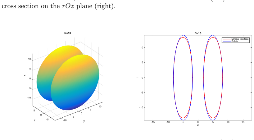
[3.1, Eq. (3.2)] After the substitution s = z/d, the dimensionless ODE should be d²r/ds² = d² [r(1+(ṙ/d)²)²/(2τ - r√(1+(ṙ/d)²))] [ρ₀/γ₀ U(ds,r) - 1/(r√(1+(ṙ/d)²))]. Equation (3.2) instead has s² and ṙ/s in place of d² and ṙ/d. As printed, (3.2) is not the transform of (3.1), so the numerical solutions labelled 'saddle interface' in Figures 4 and 6 are not solutions of the stated stationarity condition unless the code silently uses the correct coefficient.
[3.1, boundary conditions after Eq. (3.1)] The saddle BVP is underdetermined: (3.2) is a second-order ODE on s∈[0,1] with only two boundary conditions, r(0)=r_min and ṙ(1)=0, while d is an unknown parameter. A second-order ODE with an unknown parameter requires a third condition to determine the solution; the phrase 'minimum value r_min' is a property, not an equation. If the intended condition is ṙ(0)=0 (or another matching condition at the neck), it must be stated and derived from the variational principle. Without this, the one-parameter family of solutions makes the reported r_min-D curves non-unique.
[3.1, Figures 4 and 6] The paper labels the computed solutions as 'saddle interfaces' but does not verify that they are index-1 stationary points of the VISM free energy (1.8). The Euler-Lagrange equation (2.3) is a necessary condition for any stationary point; the boundary conditions used for the saddle are imposed ad hoc (r(0)=r_min, ṙ(1)=0) and are not shown to follow from the first variation of the functional. No second-variation or eigenvalue analysis is provided. As a result, the central claim that the method computes transition-state interfaces is unsupported; the computed curves may correspond to a different family of solutions of the ODE.
[3.2, boundary condition z(d)=r_max] The boundary condition is written as z(d)=r_max, where z is solved as a function of r and r_max is the maximum radial value of the connected interface. For the disconnected 'cap' to meet the connected interface at its outer edge, the condition should be z(r_max)=d, i.e., the z-coordinate at radius r_max equals d. As written, the condition equates a value of the dependent variable z at argument d to a radial coordinate r_max, which is not the geometric matching condition and is dimensionally inconsistent in its argument ordering.
[3.5, Figure 6] The threshold statements 'for D > 8.26' and 'for rmin < 1.61' are not grounded in the numerical procedure described. In the saddle computation, r_min is an input parameter and D is determined by the BVP solution; the paper does not explain how one fixes D and solves for r_min, nor does it report the domain of existence of solutions in (r_min, D) space. Without a stated root-finding or continuation procedure, these thresholds are ambiguous and cannot be reproduced.

minor comments (6)

[Throughout] The symbol '∫hortrightarrow' appears in place of an arrow in several places (e.g., Theorem 1.4, Remark 1.5, Section 3.3); this rendering error should be corrected to the intended arrow symbol.
[1.2] The phrase 'water or other fluids nearly of multiphase coexistence like' contains a grammatical error; it should read 'such as water' or similar.
[2.1] The notation r is used for both the three-dimensional distance and the cylindrical radial coordinate; although the author notes the abuse, this makes Eqs. (2.1)-(2.2) harder to follow and should be disambiguated.
[3.3, Remark 3.3] The statement 'Numerical computations suggest z̈(0)=0' is presented without evidence; if this is a numerical observation, it should be shown (e.g., a plot or table), and its use in characterizing the disconnected interface should be justified.
[3.4-3.5] The paper does not include any convergence study or details of the bvp4c implementation (tolerances, mesh refinement, initial guesses); such information is necessary for the reported numbers in Figures 3-9 to be reproducible.
[Figure 6] The right panel appears to duplicate the left panel; the caption 'Simulation of the entire rmin-D curve' should clarify what additional information it provides.

Circularity Check

1 steps flagged · score 6.0 of 10

Saddle rmin-D curve is generated by imposing the stable solution's minimum as a boundary condition, so the reported stable-saddle coincidence is built in.

fitted input called prediction [Section 3.1 (eq. (3.2) and boundary conditions) and Section 3.5 (Figure 6)]
"For the saddle solution of (3.1), inspired by [40] and noting the symmetric assumption on the interface proposed in Subsection 2.3 ... we consider the portion of the interface where its z-coordinate falls in the interval [0, d]. We use the minimum value rmin of r(z) where −d ≤ z ≤ d as boundary condition on the left, and we take d as an undetermined constant. ... Let the minimum distance from a point on the solute-solvent interface (the portion between two ellipsoidal molecules) to the z-axis be denoted by rmin."

In the saddle BVP (3.2), rmin is not an output of the computation; it is prescribed as the left boundary condition r(0)=rmin. In context, the only previously computed r(z) with a well-defined minimum is the connected minimal (stable) interface from (3.1), so the saddle branch is constructed by feeding the stable solution's minimum into the solver as an input. Section 3.5 then reports the same quantity as a numerical prediction for the saddle interface and states that the stable rmin-D curve coincides with the saddle one. That coincidence is forced by construction, not discovered: the saddle curve is the stable minimum used as a boundary condition.

full rationale

Most of the derivation is self-contained: (1.11) is the Euler-Lagrange equation of the VISM free energy (1.8), and the ODEs (3.1) and (3.4) follow from the cylindrical parameterization with no fitting to the paper's own target data. All model parameters in Table 1 are external values taken from [24,27,39]. The circularity is localized to the saddle computation: the BVP (3.2) takes r(0)=rmin as a prescribed boundary value, and the only prior rmin in the paper is the minimum of the stable connected interface. Section 3.5 then presents the rmin-D curve for the saddle and 'verifies' that the stable curve coincides with it; that coincidence is true by construction, not by numerical discovery. The saddle identification is also not checked by a second-variation/index-1 computation, and the BVP as written omits a third condition needed when d is treated as an unknown parameter, but those are correctness gaps rather than circularity. Because one numerical result central to the 'interface varies with distance' claim reduces to its own input, the paper is partially circular.

Assumptions & free parameters 1 free parameters · 6 assumptions · 0 invented entities

The paper introduces no new physical entities. Its central claim rests on imported model assumptions, on a symmetry ansatz for the interface, and on boundary conditions for the saddle solution that are imposed ad hoc. The only free parameter in the method itself is the neck radius rmin, which is an input for the saddle computation.

free parameters (1)

rmin (neck radius for saddle interface) = varied, threshold 1.61 Å
Imposed as a boundary condition r(0)=rmin in (3.2) rather than derived from the variational principle; the saddle solution family is parametrized by it, and Figure 6 reports rmin as if it were an output.

assumptions (6)

domain assumption The variational implicit solvent model of Dzubiella-Swanson-McCammon is an adequate description of sharp hydrophobic solvation interfaces.
The entire paper is built on this model, introduced in Section 1 from references [25,26]; no justification is given for why a sharp interface is valid for the two-ellipsoid system.
domain assumption The equilibrium solute-solvent interface is a surface of revolution symmetric about the z-axis and the xOy-plane.
Stated in Section 2.3 as further assumptions; this restricts the solution space and is not proven for the global minimizer or saddles.
domain assumption The pressure-volume term P Vol can be neglected during minimization.
Section 2.3 states that Gvol is neglected; this is valid only if P is small, which is discussed but not quantified for the chosen system.
domain assumption The Gay-Berne Lennard-Jones potential (2.1) correctly models the solute-solvent interaction of the ellipsoidal molecules.
Adopted from references [24,39]; the ellipsoidal shape and parameter values in Table 1 are taken as given.
ad hoc to paper The boundary conditions for the connected interface, dr/dz(±d)=0, and for the saddle interface, r(0)=rmin and dr/ds(1)=0, select the correct stationary solutions.
These conditions are imposed in Sections 3.1 and 3.2 without derivation from the variational principle; the saddle boundary condition in particular introduces rmin as a free input.
standard math Solutions of the ODE (3.4) and (3.5) with the stated boundary conditions correspond to disconnected interfaces whose intersection with the z-axis gives the quadratic equation (3.6).
The Taylor expansion argument in Section 3.3 is mathematically standard, but it assumes smoothness of z(r) at r=0.

how reviews work

0 comments

Cite this review

Pith. "Pith review of Characterizations of sharp solute-solvent interfaces in hydrophobic environments via cylindrical coordinates." pith.science (2026). https://pith.science/paper/QMDP55BZ

@misc{pith2026241213590,
  author       = {Pith},
  title        = {Pith review of: Characterizations of sharp solute-solvent interfaces in hydrophobic environments via cylindrical coordinates},
  year         = {2026},
  howpublished = {\url{https://pith.science/paper/QMDP55BZ}},
  note         = {Machine review of arXiv:2412.13590}
}

read the original abstract

This paper characterizes sharp solute-solvent interfaces in hydrophobic environments, and there are three major ingredients. The first is the variational implicit solvent model (VISM) which establishes the free energy functional of arbitrary solvation states. The minimization of this functional yields a PDE which characterizes both the stable and saddle solute-solvent interfaces. The second is a solute system consisting of two Gay-Berne ellipsoidal hydrophobic molecules. The cylindrical coordinates reduce the corresponding PDE to an ODE which is more traceable, increasing the computability of the solute-solvent interfaces under solvation effects. The third, which is the innovative part of this paper, transforms the computation of sharp solute-solvent interfaces into an ODE boundary value problem. We introduce an effective method for numerically computing saddle interfaces. This remains a hard problem in previous research. Besides, we address some qualitative results and study how the interface varies with respect to the distance between the two Gay-Berne ellipsoidal hydrophobic molecules.

Figures

Figures reproduced from arXiv: 2412.13590 by the authors.

**Figure 2.** Dual Gay-Berne ellipsoidal hydrophobic solute molecules [24]. Let u be the z-coordinate of P. The Lennard-Jones potential induced by this solvation system is U(⃗r) = U1(⃗r) + U2(⃗r) where U1(⃗r) = ULJ(r1, θ1), U2(⃗r) = ULJ(r2, θ2), r1 = p r 2 + (d + u) 2, θ1 = arctan r d + u , and r2 = p r 2 + (d − u) 2, θ2 = arctan r d − u . 2.3. Cylindrical parameterization, curvature, and free energy minimization. For the solvati… view at source ↗

**Figure 3.** For D = 10, the stable connected solute-solvent interface (left) and its cross section on the rOz plane (right). 3.5. The interface morphology varying by the distance between ellipsoidal molecules. Let the minimum distance from a point on the solute-solvent interface (the portion between two ellipsoidal molecules) to the z-axis be denoted by rmin. By numerical computations, we obtain the graph of rmin varying with r… view at source ↗

Figures from the paper (6 more)

**Figure 4.** Figure 4: For D = 10, the saddle connected solute-solvent interface (left) and its cross section on the rOz plane (right). z -15 -10 -5 0 5 10 15 r -10 -5 0 5 10 D=10 Minimal Interface Solute [PITH_FULL_IMAGE:figures/full_fig_p014_4.png]

**Figure 5.** Figure 5: For D = 10, the stable disconnected solute-solvent interface (left) and its cross section on the rOz plane (right). In numerical computations, we found that, when accurate to two decimal places for D > 8.26, the system no longer has a connected solute-solvent interface…

**Figure 6.** Figure 6: The varying trend of rmin with respect to D (left); Simulation of the entire rmin-D curve of the saddle interface (right) where the stable one coincides with the upper half of the saddle one. the region W of the entire system as a cylinder with L = 50, i.e. W :    x…

**Figure 7.** Figure 7: The varying trend of Garea with respect to D (left); The varying trend of Gmean with respect to D (right). D 9 10 11 12 13 14 15 Energy 150 200 250 300 350 400 G geo Connected Minimal Interface Connected Saddle Interface Disconnected Minimal Interface D 9 10 11 12 13 1…

**Figure 8.** Figure 8: The varying trend of Ggeo with respect to D (left); The varying trend of GvdW with respect to D (right). [5] K. Leung, A. Luzar, and D. Bratko, Dynamics of Capillary Drying in Water, Phys. Rev. Lett. 90 (2003), 065502. [6] K. Lum and A. Luzar, Pathway to surface-induce…

**Figure 9.** Figure 9: The varying trend of Gtot with respect to D. [10] C. L. Brooks, M. Gruebele, J. N. Onuchic, and P. G. Wolynes, Chemical physics of protein folding, Proc. Natl. Acad. Sci. USA 95 (1998), 11037–11038. [11] L. R. Pratt and D. Chandler, Theory of the hydrophobic effect, J.…

Discussion (0). Continue with ORCID to comment.

Reference graph

Works this paper leans on

41 extracted references · 41 canonical work pages

[1]

Ball, Chemical physics: How to keep dry in water , Nature 423 (2003), 25–26

P. Ball, Chemical physics: How to keep dry in water , Nature 423 (2003), 25–26

work page 2003
[2]

Hummer, S

G. Hummer, S. Garde, A. E. Garc ´ ıa, and L. R. Pratt, New perspectives on hydrophobic effects , Chem. Phys. 258 (2000), 349–370

work page 2000
[3]

Luzar and K

A. Luzar and K. Leung, Dynamics of capillary evaporation. I. Effect of morphology of hydrophobic surfaces , J. Chem. Phys. 113 (2000), 5836–5844

work page 2000
[4]

Leung and A

K. Leung and A. Luzar, Dynamics of capillary evaporation. II. Free energy barriers, J. Chem. Phys. 113 (2000), 5845–5852. 16 HAO XIAO D 9 10 11 12 13 14 15 Energy 200 250 300 350 400 450 500 Garea Connected Minimal Interface Connected Saddle Interface Disconnected Minimal Interface D 9 10 11 12 13 14 15 Energy -75 -70 -65 -60 -55 -50 -45 -40 -35 Gmean Con...

work page 2000
[5]

Leung, A

K. Leung, A. Luzar, and D. Bratko, Dynamics of Capillary Drying in Water , Phys. Rev. Lett. 90 (2003), 065502

work page 2003
[6]

Lum and A

K. Lum and A. Luzar, Pathway to surface-induced phase transition of a confined fluid , Phys. Rev. E 56 (1997), R6283–R6286

work page 1997
[7]

A. R. Fersht, Structure and mechanism in protein science , W. H. Freeman, New York, 1999

work page 1999
[8]

C. L. Brooks, J. N. Onuchic, and D. J. Wales, Statistical thermodynamics: Taking a walk on a landscape, Science 293 (2001), 612–613

work page 2001

Show all 41 references

[9]

C. M. Dobson, A. ˇSali, and M. Karplus, Protein folding: A perspective from theory and experiment , Angew. Chem. Int. Ed. Engl. 37 (1998), 868–893. CHARACTERIZATIONS OF SHARP SOLUTE-SOL VENT INTERF ACES 17 D 9 10 11 12 13 14 15 Energy 150 200 250 300 350 400 Gtot Connected Min...

1998
[10]

C. L. Brooks, M. Gruebele, J. N. Onuchic, and P. G. Wolynes, Chemical physics of protein folding , Proc. Natl. Acad. Sci. USA 95 (1998), 11037–11038

1998
[11]

L. R. Pratt and D. Chandler, Theory of the hydrophobic effect , J. Chem. Phys. 67 (1977), 3683–3704

1977
[12]

Chandler, Hydrophobicity: Two faces of water , Nature 417 (2002), 491

D. Chandler, Hydrophobicity: Two faces of water , Nature 417 (2002), 491

2002
[13]

F. H. Stillinger, Structure in aqueous solutions of nonpolar solutes from the standpoint of scaled-particle theory , J. Solution Chem. 2 (1973), 141-–158

1973
[14]

Pangali, M

C. Pangali, M. Rao, and B. J. Berne, Hydrophobic hydration around a pair of apolar species in water , J. Chem. Phys. 71 (1979), 2982—2990

1979
[15]

Pangali, M

C. Pangali, M. Rao, and B. J. Berne, A Monte Carlo simulation of the hydrophobic interaction , J. Chem. Phys. 71 (1979), 2975-–2981

1979
[16]

Huang, C

X. Huang, C. J. Margulis, and B. J. Berne, Do molecules as small as neopentane induce a hydrophobic response similar to that of large hydrophobic surfaces? , J. Phys. Chem. B (2003), 11742–11748

2003
[17]

C. Y. Lee, J. A. McCammon, and P. J. Rossky, The structure of liquid water at an extended hydrophobic surface , J. Chem. Phys. 80 (1984), 4448—4455

1984
[18]

Y. K. Cheng and P. J. Rossky, Surface topography dependence of biomolecular hydrophobic hydration , Nature 392 (1998), 696–699

1998
[19]

T. R. Jensen, M. Ø. Jensen, N. Reitzel, K. Balashev, G. H. Peters, K. Kjaer, and T. Bjørnholm, Water in contact with extended hydrophobic surfaces: Direct evidence of weak dewetting , Phys. Rev. Lett. 90 (2003), 086101

2003
[20]

K. Lum, D. Chandler, and J. D. Weeks, Hydrophobicity at small and large length scales , J. Phys. Chem. B 103 (1999), 4570—4577. 18 HAO XIAO

1999
[21]

D. M. Huang and D. Chandler, The hydrophobic effect and the influence of solute-solvent attractions , J. Phys. Chem. B 106 (2002), 2047–2053

2002
[22]

Wallqvist and B

A. Wallqvist and B. J. Berne, Molecular dynamics study of the dependence of water solvation free energy on solute curvature and surface area , J. Phys. Chem. 99 (1995), 2885-–2892

1995
[23]

Wallqvist and B

A. Wallqvist and B. J. Berne, Computer simulation of hydrophobic hydration forces on stacked plates at short range J. Phys. Chem. 99 (1995), 2893—2899

1995
[24]

Huang, C

X. Huang, C. J. Margulis, and B. J. Berne, Dewetting-induced collapse of hydrophobic particles , Proc. Natl. Acad. Sci. USA 100 (2003), 11953–11958

2003
[25]

Dzubiella, J

J. Dzubiella, J. M. J. Swanson, and J. A. McCammon, Coupling hydrophobicity, dispersion, and electrostatics in continuum solvent models , Phys. Rev. Lett. 96 (2006), 087802

2006
[26]

Dzubiella, J

J. Dzubiella, J. M. J. Swanson, and J. A. McCammon, Coupling nonpolar and polar solvation free energies in implicit solvent models , J. Chem. Phys. 124 (2006), 084905

2006
[27]

L. T. Cheng, J. Dzubiella, J. A. McCammon, and B. Li, Application of the level-set method to the implicit solvation of nonpolar molecules , J. Chem. Phys. 127 (2007), 084503

2007
[28]

Chandler, Interfaces and the driving force of hydrophobic assembly , Nature 437 (2005), 640–647

D. Chandler, Interfaces and the driving force of hydrophobic assembly , Nature 437 (2005), 640–647

2005
[29]

D. G. Triezenberg and R. Zwanzig, Fluctuation theory of surface tension Phys. Rev. Lett. 28 (1972), 1183

1972
[30]

Reiss, Scaled particle methods in the statistical thermodynamics of fluids Adv

H. Reiss, Scaled particle methods in the statistical thermodynamics of fluids Adv. Chem. Phys. 9 (1965), 1–84

1965
[31]

R. C. Tolman, The effect of droplet size on surface tension J. Chem. Phys. 17 (1949), 333—337

1949
[32]

D. M. Huang, P. L. Geissler, and D. Chandler, Scaling of hydrophobic solvation free energies J. Phys. Chem. B 105 (2001), 6704—6709

2001
[33]

Hadwiger, Vorlesungen ¨Uber Inhalt, Oberfl¨ ache und Isoperimetrie , Springer-Verlag, Berlin-G¨ ottingen- Heidelberg, 1975

H. Hadwiger, Vorlesungen ¨Uber Inhalt, Oberfl¨ ache und Isoperimetrie , Springer-Verlag, Berlin-G¨ ottingen- Heidelberg, 1975

1975
[34]

M. P. do Carmo, Differential geometry of curves & surfaces , Dover Publications Inc., USA, 2016

2016
[35]

O. Y. Zhong-can and W. Helfrich, Bending energy of vesicle membranes: General expressions for the first, second, and third variation of the shape energy and applications to spheres and cylinders , Phys. Rev. A 39 (1989), 5280–5288

1989
[36]

N. C. Overgaard and J. E. Solem, The variational origin of motion by Gaussian curvature , In: F. Sgallari, A. Murli, and N. Paragios (eds), Scale space and variational methods in computer vision , Lecture Notes in Computer Science 4485, Springer-Verlag, Berlin-Heidelberg, 2007...

2007
[37]

Spivak, A comprehensive introduction to differential geometry: Vol

M. Spivak, A comprehensive introduction to differential geometry: Vol. 4 , Publish or Perish, USA, 1999, pp. 259–281

1999
[38]

L. D. Landau and E. M. Lifshitz, Mechanics, Butterworth-Heinemann, India, 1976

1976
[39]

Huang, R

X. Huang, R. Zhou, and B. J. Berne, Drying and hydrophobic collapse of paraffin plates , J. Phys. Chem. B 109 (2005), 3546—3552

2005
[40]

J. Ding, H. Sun, Z. Wang, and S. Zhou, Computational study on hysteresis of ion channels: Multiple solutions to steady-state Poisson-Nernst-Planck equations , Commun. Comput. Phys. 23 (2018), 1549–1572

2018
[41]

L. F. Shampine, M. W. Reichelt, and J. Kierzenka, Solving boundary value problems for ordinary differential equations in MATLAB with bvp4c , Tutorial Notes, 2000. (Previous) School of Mathematical Sciences, Soochow University, Suzhou, Jiangsu 215006, China Email address : hxia...

2000

Pith tools

Reviewed August 11, 2026 · model on record in the stance chip above.

[1] [1]

Ball, Chemical physics: How to keep dry in water , Nature 423 (2003), 25–26

P. Ball, Chemical physics: How to keep dry in water , Nature 423 (2003), 25–26

work page 2003

[2] [2]

Hummer, S

G. Hummer, S. Garde, A. E. Garc ´ ıa, and L. R. Pratt, New perspectives on hydrophobic effects , Chem. Phys. 258 (2000), 349–370

work page 2000

[3] [3]

Luzar and K

A. Luzar and K. Leung, Dynamics of capillary evaporation. I. Effect of morphology of hydrophobic surfaces , J. Chem. Phys. 113 (2000), 5836–5844

work page 2000

[4] [4]

Leung and A

K. Leung and A. Luzar, Dynamics of capillary evaporation. II. Free energy barriers, J. Chem. Phys. 113 (2000), 5845–5852. 16 HAO XIAO D 9 10 11 12 13 14 15 Energy 200 250 300 350 400 450 500 Garea Connected Minimal Interface Connected Saddle Interface Disconnected Minimal Interface D 9 10 11 12 13 14 15 Energy -75 -70 -65 -60 -55 -50 -45 -40 -35 Gmean Con...

work page 2000

[5] [5]

Leung, A

K. Leung, A. Luzar, and D. Bratko, Dynamics of Capillary Drying in Water , Phys. Rev. Lett. 90 (2003), 065502

work page 2003

[6] [6]

Lum and A

K. Lum and A. Luzar, Pathway to surface-induced phase transition of a confined fluid , Phys. Rev. E 56 (1997), R6283–R6286

work page 1997

[7] [7]

A. R. Fersht, Structure and mechanism in protein science , W. H. Freeman, New York, 1999

work page 1999

[8] [8]

C. L. Brooks, J. N. Onuchic, and D. J. Wales, Statistical thermodynamics: Taking a walk on a landscape, Science 293 (2001), 612–613

work page 2001