REVIEW 4 major objections 5 minor 62 references
Stroboscopic measurements in Markov networks: Exact generator reconstruction vs. thermodynamic inference
T0 review · 4 major / 5 minor · reviewed 2026-08-11 · deepseek-v4-flash
Pith's one-line read Below a critical sampling rate, stroboscopic snapshots recover the full generator.
desk verdict A sound and honest compilation of known generator-uniqueness results with a genuinely useful new bounding method, weakened mainly by the infinite-data idealization and the absence of finite-sample error analysis. read the letter →
The pith
A machine-rendered reading of the paper's core claim, the machinery that carries it, and where it could break.
The reading
What carries the argument
The load-bearing identity is the matrix exponential $G_{\Delta t}=e^{\Delta t L_0}$ together with the classification of all matrices whose exponential equals $G_{\Delta t}$. The proof uses the Gerschgorin circle theorem to show that any permissible generator has all eigenvalues inside a disc of radius $r_{\max}$ centered at $-r_{\max}$, so eigenvalues shifted by $2\pi i/\Delta t$ leave the allowed region whenever $r_{\max}<\pi/\Delta t$; this forces $J=0$ in the logarithm formula and makes the principal-branch logarithm the unique answer. The operationally accessible version replaces the unknown $r_{\max}$ with an upper bound $r_{\max}^{\mathrm{ub}}$ derived from the propagator's diagonal entries and the trace identity. This machinery both proves exact recovery below the threshold and parametrizes the finite candidate set above it.
What would settle it
A decisive numerical check of the claimed threshold: for the four-state cyclic generator family of Appendix A, set $\Delta t=\pi/r+\varepsilon$ with $\varepsilon>0$ and verify that $L_0$ and $L_0^T$ are distinct permissible generators with the same propagator; then set $\Delta t=\pi/r-\varepsilon$ and exhaustively search the integer-shift family for a second permissible generator with $r_{\max}<\pi/\Delta t$. Finding none below the threshold confirms the bound is tight; finding one would refute the uniqueness theorem.
Extended reading notes
Core claim
For a continuous-time Markov jump process on a connected network observed at fixed intervals $\Delta t$, the paper proves that a permissible generator $L_0$ satisfying $\exp(\Delta t L_0)=G_{\Delta t}$ and $r_{\max}(L_0)<\pi/\Delta t$ is unique and is constructively recovered as $L_0 = \frac{1}{\Delta t} Z \ln(D) Z^{-1}$ from a diagonalization $G_{\Delta t}=Z D Z^{-1}$. Since $r_{\max}$ is not directly observable, the paper derives the operational criterion $r_{\max}^{\mathrm{ub}}<\pi/\Delta t$, computed from the diagonal of $G_{\Delta t}$ and the trace identity $\sum_i r_i=-\ln\det(G_{\Delta t})/\Delta t$, that guarantees the uniqueness condition is met. When the criterion fails and the eigenvalues of $G_{\Delta t}$ are non-degenerate, all candidate generators take the form $L_J = Z\big(\frac{1}{\Delta t}\ln D + \frac{2\pi i}{\Delta t}\operatorname{diag}(j_1,\dots,j_N)\big)Z^{-1}$ with finitely many integer vectors $J$; evaluating thermodynamic quantities over the permissible candidates gives tight upper and lower bounds, which is an original contribution relative to the existing literature.
Load-bearing premise
The proof assumes the propagator $G_{\Delta t}$ is known exactly, i.e., infinite stroboscopic data; with finite sampling, the matrix logarithm becomes unstable precisely in the regime where exact recovery is claimed, and the paper does not analyze that error propagation.
Editorial extensions
If this is right
- For $\Delta t<\pi/r_{\max}^{\mathrm{ub}}$, all transition rates, the mean entropy production rate, and every cycle affinity are determined exactly from stroboscopic data; no lower-bound estimator is needed.
- The threshold $\pi/r_{\max}^{\mathrm{ub}}$ is computable from the observed propagator alone, so an experimenter can know from the data whether exact inference is guaranteed.
- Above the threshold, in the generic non-degenerate case, the minimum and maximum of any rate-dependent thermodynamic quantity over the finite candidate set are tight bounds that improve on the KL-divergence estimator $\hat{\sigma}$.
- If $G_{\Delta t}$ has real pairwise distinct eigenvalues, the generator is unique for every $\Delta t$; in particular, two-state systems are always exactly reconstructible.
- For cycle affinities the method yields individual lower and upper bounds for every cycle, whereas the compared extant estimator offers only a single lower bound on the largest affinity.
Reading between the lines
- The paper's exactness claim assumes an exactly known propagator; for finite data, errors in $G_{\Delta t}$ propagate through the matrix logarithm and are likely to be severe near $\Delta t=\pi/r_{\max}$, so practical implementations will need regularization or uncertainty quantification that the paper does not provide.
- Because the full generator is recovered below threshold, the same reconstruction could feed any generator-dependent thermodynamic or kinetic quantity, not only entropy production and affinities, for example current fluctuations or average traffic.
- Degenerate eigenvalues break the finite-enumeration argument and can yield uncountably many candidate generators; detecting near-degeneracies from data and deciding how to bound thermodynamics in that case is an open problem the paper only flags implicitly.
- The threshold has a physical reading: strobes must be faster than the fastest escape timescale. This suggests a practical protocol, shorten $\Delta t$ until $r_{\max}^{\mathrm{ub}}\Delta t/\pi<1$, that makes exact inference a tunable experimental resource rather than a fixed property of the system.
Signed reviews
Editorial analysis
A structured set of objections, weighed in public.
Referee Report
Summary. The paper studies whether a continuous-time Markov generator on a finite network can be reconstructed from stroboscopic observations of the propagator G_Δt = exp(Δt L0). Section 3.1 proves that if a permissible generator satisfies rmax(L0) < π/Δt, then it is the unique generator for that propagator and can be obtained constructively via the principal matrix logarithm. Section 3.2 replaces the inaccessible condition on rmax with operationally checkable sufficient criteria, in particular the bound rub_max < π/Δt, and Section 3.3 enumerates finitely many candidate generators in the generic nondegenerate case, yielding upper and lower bounds on thermodynamic quantities such as entropy production and cycle affinities. Section 4 compares this approach with a Kullback-Leibler-based entropy estimator and a conjectured affinity bound, using numerical illustrations on three small networks. The paper explicitly works under the idealized assumption of infinite data, and it also acknowledges several limitations, including the non-generic degenerate case and the absence of a full finite-sample analysis.
Significance. If the main theorem is correct, the paper makes a useful conceptual contribution: below an operationally detectable threshold in Δt, stroboscopic data determine the full generator and hence all thermodynamic quantities, not merely lower bounds. The proof of the uniqueness statement is self-contained, anchored in established results (Gerschgorin's theorem and Higham's matrix-logarithm theorems), and introduces no fitted parameters. The finite-candidate enumeration and the resulting tight bounds are a genuine extension beyond exact reconstruction. The numerical demonstrations support the claims in the idealized setting, but the practical significance is attenuated by the lack of finite-data error analysis and by the fact that the numerical candidate enumeration is performed from the true generator rather than from an estimated propagator.
major comments (4)
- [Section 2 and Section 4.1] The paper explicitly assumes 'in principle infinite data' in Section 2, but the abstract and the numerical comparison frame the method as a practical inference tool for stroboscopic measurements. No error analysis is provided for an empirically estimated G_Δt. The matrix logarithm is discontinuous when an eigenvalue of G_Δt approaches the negative real axis, and this is precisely the regime relevant when rmax is close to π/Δt; a small statistical fluctuation can shift an eigenvalue across the branch cut and change the reconstructed generator by 2πi/Δt, with correspondingly large errors in rates, entropy production, and affinities. Moreover, the criterion rub_max < π/Δt is itself evaluated from the noisy propagator, so it can be satisfied or violated by chance without any confidence guarantee. I request either a finite-sample error propagation analysis or an explicit restriction of the exactness and tightness claims to the infinite-data idealization throughout the abstract and conclusions.
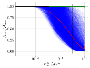
- [Section 4.1, Figure 3, Figure 4] The numerical validation does not test the proposed inference pipeline end-to-end. The text states that 'we can compute all other candidate generators LJ directly from the randomly generated L0 rather than GΔt, which reduces numerical errors.' Thus the candidate set and the reported bounds are constructed from the true generator, bypassing both the matrix logarithm and the operationally accessible bound rub_max that the method is supposed to use. The comparison against the estimators (36) and (38) therefore illustrates ideal mathematical bounds rather than the performance of the proposed procedure on estimated propagators. Please rerun the numerics with empirical transition matrices, or state clearly in the figure captions and Section 4 that these plots assume exact knowledge of the propagator.
- [Section 3.3, Eqs. (34)-(39)] The abstract says that beyond the critical interval 'we still obtain tight upper and lower bounds on these quantities that improve on extant methods.' Within the paper this claim is explicitly restricted to the generic case of pairwise nondegenerate eigenvalues of G_Δt; Section 3.3 acknowledges that degenerate eigenvalues can give uncountably many candidate generators and break the finite-enumeration bounds. Since this is a load-bearing qualification, the abstract and the summary of the main results should state the nondegeneracy assumption explicitly rather than presenting the bounds as unconditional. The scaling estimate (39) also relies on rub_max ≤ N rmax and on the number of non-real simple eigenvalues; the text should clarify the sense in which this is only a crude upper estimate.
- [Section 4.2, Eq. (38)] The improved affinity bound (38) is labeled as conjectured and is supported only by numerical evidence for a particular four-state network. The comparison in Figure 4 uses this conjectured estimator as a benchmark, so the claim that the proposed bounds 'improve on extant methods' is conditional on a statement that has not been proved. If (38) fails for other topologies or parameter ranges, the demonstrated improvement over extant affinity estimators may not hold. At minimum, the comparison should report the dependence of the benchmark on the conjecture, or use a provable bound instead.
minor comments (5)
- [Section 2, after Eq. (7)] There is a typo: 'the state of the system system is measured' should read 'the state of the system is measured'.
- [Section 3.2.1, Eqs. (27)-(28)] The criterion (27) is derived in the text through Eqs. (21)-(26), but the improved criterion (28) is cited to Cuthbert without proof. Since the paper aims to be self-contained, a proof or a statement that (28) is used only as an optional refinement would help; as written, the reader cannot verify the claimed improvement without consulting Ref. [45].
- [Figure caption of Figure 3] The phrase '10 5 configurations' appears with a missing superscript; it should be '10^5 configurations'. The same issue occurs in the caption of Figure 4.
- [Throughout, especially Section 3.1] The spelling 'Gerschgorin' is used consistently, but the standard English transliteration is 'Gershgorin'; the authors may wish to align with the reference list or add a parenthetical note.
- [Section 4.1, paragraph after Eq. (36)] The quantity (36) is first introduced as a Kullback-Leibler divergence but then called the 'quality factor' in the figures; please define the quality factor explicitly in the main text rather than only in the figure captions.
Circularity Check
No circular derivation: the uniqueness theorem and reconstruction formula are proved from external matrix-logarithm and Gerschgorin results, with no fitted parameter renamed as a prediction.
full rationale
The central reconstruction claim (Section 3.1) is proved from Gerschgorin's theorem and Higham's classification of matrix logarithms; the condition rmax(L0)<pi/dt is a generator property, not an inferred quantity. The operational criterion rub_max<pi/dt (Section 3.2.1) is a genuine sufficient condition derived from path-weight inequalities and det(Gdt)=exp(Tr L0 dt), not a fitted parameter renamed as a prediction. Section 3.3 enumerates all matrices satisfying exp(dt LJ)=Gdt and permissibility, so the resulting bounds are tight by construction over the model class. The affinity conjecture (38) is explicitly presented as a conjecture, not as a derived prediction. Self-citations appear only for comparison estimators and background and are not load-bearing for the uniqueness or bounding proofs. The numerical shortcut of computing candidates from the true L0 rather than Gdt is an implementation detail, not a circular step. Hence the paper's derivation is self-contained and non-circular; the only minor caveat is non-load-bearing self-citation in the comparison sections.
Assumptions & free parameters
assumptions (6)
- standard math Gerschgorin circle theorem
- standard math Higham's Theorem 1.27 on the general form of matrix logarithms
- standard math Frobenius theorem: irreducible nonnegative matrices have a simple Perron eigenvalue
- domain assumption The underlying system is a continuous-time Markov chain on a finite connected network with unique stationary state and bidirectional transitions
- domain assumption Infinite data idealization: propagator GΔt is known exactly
- domain assumption Non-degenerate eigenvalues of GΔt in the general case (Section 3.3)
Cite this review
Pith. "Pith review of Stroboscopic measurements in Markov networks: Exact generator reconstruction vs. thermodynamic inference." pith.science (2026). https://pith.science/paper/LBAFRIVB
@misc{pith2026241215642,
  author       = {Pith},
  title        = {Pith review of: Stroboscopic measurements in Markov networks: Exact generator reconstruction vs. thermodynamic inference},
  year         = {2026},
  howpublished = {\url{https://pith.science/paper/LBAFRIVB}},
  note         = {Machine review of arXiv:2412.15642}
}
read the original abstract
A major goal of stochastic thermodynamics is to estimate the inevitable dissipation that accompanies particular observable phenomena in an otherwise not fully accessible system. Quantitative results are often formulated as lower bounds on the total entropy production, which capture the part of the total dissipation that can be determined based on the available data alone. In this work, we discuss the case of a continuous-time dynamics on a Markov network that is observed stroboscopically, i.e., at discrete points in time in regular intervals. We compare the standard approach of deriving a lower bound on the entropy production rate in the steady state to the less common method of reconstructing the generator from the observed propagators by taking the matrix logarithm. Provided that the timescale of the stroboscopic measurements is smaller than a critical value that can be determined from the available data, this latter method is able to recover all thermodynamic quantities like entropy production or cycle affinities and is therefore superior to the usual approach of deriving lower bounds. Beyond the critical value, we still obtain tight upper and lower bounds on these quantities that improve on extant methods. We conclude the comparison with numerical illustrations and a discussion of the requirements and limitations of both methods.
Figures


Figures from the paper (2 more)

Reference graph
Works this paper leans on
-
[1]
Seifert U 2012 Stochastic thermodynamics, fluctuation theorems, and molecular machines Rep. Prog. Phys. 75 126001
work page 2012
-
[2]
van den Broeck C and Esposito M 2015 Ensemble and trajectory thermodynamics: A brief intro- duction Physica A 418 6 – 16
work page 2015
-
[3]
An Introduction (Princeton Univ
Peliti L and Pigolotti S 2021 Stochastic thermodynamics. An Introduction (Princeton Univ. Press)
work page 2021
-
[4]
Shiraishi N 2023 An introduction to stochastic thermodynamics 1st ed Fundamental Theories of Physics (Singapore, Singapore: Springer)
work page 2023
-
[5]
Seifert U 2019 From stochastic thermodynamics to thermodynamic inference Ann. Rev. Cond. Mat. Phys. 10 171–192
work page 2019
-
[6]
Barato A C and Seifert U 2015 Thermodynamic uncertainty relation for biomolecular processes Phys. Rev. Lett. 114(15) 158101
work page 2015
-
[7]
Gingrich T R, Horowitz J M, Perunov N and England J L 2016 Dissipation bounds all steady-state current fluctuations Phys. Rev. Lett. 116(12) 120601
work page 2016
-
[8]
Horowitz J M and Gingrich T R 2020 Thermodynamic uncertainty relations constrain non- equilibrium fluctuations Nat. Phys. 16 15–20
work page 2020
Show all 62 references
-
[9]
Kawai R, Parrondo J M R and van den Broeck C 2007 Dissipation: The phase-space perspective Phys. Rev. Lett. 98 080602
2007
-
[10]
Gomez-Marin A, Parrondo J M R and Van den Broeck C 2008 Lower bounds on dissipation upon coarse-graining Phys. Rev. E 78 011107
2008
-
[11]
Gomez-Marin A, Parrondo J and van den Broeck C 2008 The ”footprints” of irreversibility EPL 82 50002
2008
-
[12]
Roldan E and Parrondo J M R 2010 Estimating dissipation from single stationary trajectories Phys. Rev. Lett. 105 150607
2010
-
[13]
Cover T M and Thomas J A 2006 Elements of information theory Telecommunications and signal processing (Hoboken, NJ, and Canada: Wiley)
2006
-
[14]
Esposito M 2012 Stochastic thermodynamics under coarse-graining Phys. Rev. E 85 041125
2012
-
[15]
Shiraishi N and Sagawa T 2015 Fluctuation theorem for partially masked nonequilibrium dynamics Phys. Rev. E 91 012130
2015
-
[16]
Bisker G, Polettini M, Gingrich T R and Horowitz J M 2017 Hierarchical bounds on entropy pro- duction inferred from partial information J. Stat. Mech. Theor. Exp. 2017 093210
2017
-
[17]
Polettini M and Esposito M 2017 Effective thermodynamics for a marginal observer Phys. Rev. Lett. 119(24) 240601
2017
-
[18]
Deg¨ unther J, van der Meer J and Seifert U 2024 Fluctuating entropy production on the coarse-grained level: Inference and localization of irreversibility Phys. Rev. Res. 6(2) 023175
2024
-
[19]
Mart ´ ınez I A, Bisker G, Horowitz J M and Parrondo J M R 2019 Inferring broken detailed balance in the absence of observable currents Nature Communications 10 3542
2019
-
[20]
van der Meer J, Ertel B and Seifert U 2022 Thermodynamic inference in partially accessible markov networks: A unifying perspective from transition-based waiting time distributions Phys. Rev. X 12 031025
2022
-
[21]
Harunari P, Dutta A, Polettini M and Roldan E 2022 What to learn from a few visible transitions’ statistics? Phys. Rev. X 12 041026
2022
-
[22]
van der Meer J, Deg¨ unther J and Seifert U 2023 Time-resolved statistics of snippets as general framework for model-free entropy estimators Phys. Rev. Lett. 130(25) 257101
2023
-
[23]
Blom K, Song K, Vouga E, Godec A and Makarov D E 2024 Milestoning estimators of dissipation in systems observed at a coarse resolution Proceedings of the National Academy of Sciences 121 e2318333121
2024
-
[24]
Deg¨ unther J, van der Meer J and Seifert U 2024 General theory for localizing the where and when of entropy production meets single-molecule experiments Proceedings of the National Academy of Sciences 121 e2405371121
2024
-
[25]
Kapustin U, Ghosal A and Bisker G 2024 Utilizing time-series measurements for entropy-production estimation in partially observed systems Phys. Rev. Res. 6(2) 023039
2024
-
[26]
Skinner D J and Dunkel J 2021 Estimating entropy production from waiting time distributions Phys. Rev. Lett. 127(19) 198101
2021
-
[27]
Pietzonka P and Coghi F 2024 Thermodynamic cost for precision of general counting observables Phys. Rev. E 109(6) 064128
2024
-
[28]
Skinner D J and Dunkel J 2021 Improved bounds on entropy production in living systems Proc. Natl. Acad. Sci. U.S.A. 118 e2024300118
2021
-
[29]
Ohga N, Ito S and Kolchinsky A 2023 Thermodynamic bound on the asymmetry of cross-correlations Phys. Rev. Lett. 131(7) 077101
2023
-
[30]
Shiraishi N 2023 Entropy production limits all fluctuation oscillations Phys. Rev. E 108(4) L042103
2023
-
[31]
Vu T V, Vo V T and Saito K 2024 Dissipation, quantum coherence, and asymmetry of finite-time cross-correlations Phys. Rev. Res. 6(1) 013273
2024
-
[32]
Dechant A, Garnier-Brun J and Sasa S i 2023 Thermodynamic bounds on correlation times Phys. Rev. Lett. 131(16) 167101
2023
-
[33]
Kolchinsky A, Ohga N and Ito S 2024 Thermodynamic bound on spectral perturbations, with ap- plications to oscillations and relaxation dynamics Phys. Rev. Res. 6(1) 013082
2024
-
[34]
Lucente D, Puglisi A, Viale M and Vulpiani A 2023 Statistical features of systems driven by non- gaussian processes: theory & practice Journal of Statistical Mechanics: Theory and Experiment 2023 113202
2023
-
[35]
Shiraishi N 2017 Finite-time thermodynamic uncertainty relation do not hold for discrete-time Markov process arXiv:1706.00892
2017 arXiv
-
[36]
Proesmans K and van den Broeck C 2017 Discrete-time thermodynamic uncertainty relation EPL 119 20001
2017
-
[37]
Chiuchi` u D and Pigolotti S 2018 Mapping of uncertainty relations between continuous and discrete time Phys. Rev. E 97(3) 032109
2018
-
[38]
Ertel B, van der Meer J and Seifert U 2022 Operationally accessible uncertainty relations for ther- modynamically consistent semi-markov processes Phys. Rev. E 105 044113
2022
-
[39]
Andrieux D and Gaspard P 2008 The fluctuation theorem for currents in semi-markov processes Journal of Statistical Mechanics: Theory and Experiment 2008 P11007
2008
-
[40]
Cisneros F A, Fakhri N and Horowitz J M 2023 Dissipative timescales from coarse-graining irre- versibility Journal of Statistical Mechanics: Theory and Experiment 2023 073201
2023
-
[41]
Liang S and Pigolotti S 2023 Thermodynamic bounds on time-reversal asymmetry Phys. Rev. E 108(6) L062101
2023
-
[42]
Elfving G 1937 Zur Theorie der Markoffschen Ketten (Helsinki: Societas scientiarum Fennica)
1937
-
[43]
Kingman J F C 1962 The imbedding problem for finite markov chains Zeitschrift f¨ ur Wahrschein- lichkeitstheorie und Verwandte Gebiete 1 14–24
1962
-
[44]
Cuthbert J R 1972 On uniqueness of the logarithm for markov semi-groups Journal of the London Mathematical Society s2-4 623–630
1972
-
[45]
Cuthbert J R 1973 The logarithm function for finite-state markov semi-groups Journal of the London Mathematical Society s2-6 524–532
1973
-
[46]
Johansen S 1974 Some results on the imbedding problem for finite markov chains Journal of the London Mathematical Society s2-8 345–351
1974
-
[47]
Israel R B, Rosenthal J S and Wei J Z 2001 Finding generators for markov chains via empirical transition matrices, with applications to credit ratings Mathematical Finance 11 245–265
2001
-
[48]
Coleman J 1973 The Mathematics of Collective Action Methodological perspectives (Chicago: Aldine Publishing Company) ISBN 9780202302584
1973
-
[49]
Singer B and Spilerman S 1973 Social mobility models for heterogeneous populations Sociological Methodology 5 356–401
1973
-
[50]
Singer B and Spilerman S 1976 The representation of social processes by markov models American Journal of Sociology 82 1–54
1976
-
[51]
Series B (Statistical Methodology) 67 395–410
Bladt M and Sørensen M 2005 Statistical inference for discretely observed markov jump processes Journal of the Royal Statistical Society. Series B (Statistical Methodology) 67 395–410
2005
-
[52]
Metzner P, Dittmer E, Jahnke T and Sch¨ utte C 2007 Generator estimation of markov jump processes Journal of Computational Physics 227 353–375
2007
-
[53]
Metzner P, Horenko I and Sch¨ utte C 2007 Generator estimation of markov jump processes based on incomplete observations nonequidistant in time Phys. Rev. E 76(6) 066702
2007
-
[54]
Verbyla K L, Yap V B, Pahwa A, Shao Y and Huttley G A 2013 The embedding problem for markov models of nucleotide substitution PLOS ONE 8 1–12
2013
-
[55]
Jia C 2016 A solution to the reversible embedding problem for finite markov chains Statistics & Probability Letters 116 122–130
2016
-
[56]
Knoch F and Speck T 2019 Non-equilibrium markov state modeling of periodically driven biomolecules The Journal of Chemical Physics 150 054103
2019
-
[57]
Gerschgorin S 1931 ¨Uber die Abgrenzung der Eigenwerte einer Matrix Izvestija Akademii Nauk SSSR, Serija Matematika 7(6) 749–754
1931
-
[58]
Higham N J 2008 Functions of Matrices (Philadelphia: Society for Industrial and Applied Mathe- matics)
2008
-
[59]
Amann C P, Schmiedl T and Seifert U 2010 Can one identify nonequilibrium in a three-state system by analyzing two-state trajectories? J. Chem. Phys. 132 041102
2010
-
[60]
Lucente D, Baldassarri A, Puglisi A, Vulpiani A and Viale M 2022 Inference of time irreversibility from incomplete information: Linear systems and its pitfalls Physical Review Research 4 043103
2022
-
[61]
Dieball C and Godec A 2024 Perspective: Time irreversibility in systems observed at coarse resolution arXiv:2412.02675
2024 arXiv
-
[62]
Barato A C and Seifert U 2017 Coherence of biochemical oscillations is bounded by driving force and network topology Phys. Rev. E 95(6) 062409
2017
Reviewed August 11, 2026 · model on record in the stance chip above.
Discussion (0). Continue with ORCID to comment.