REVIEW 4 major objections 6 minor 18 references
Fuzzy-Space Engineering
T0 review · 4 major / 6 minor · reviewed 2026-08-11 · deepseek-v4-flash
Pith's one-line read The paper claims that a 30-node graph shaped like a Trefoil knot, encoded into three hermitian matrices, yields a zero-mode surface whose real locus is a two-dimensional Trefoil knot embedded in R^3.
desk verdict A practical visualization toolkit for fuzzy zero-mode surfaces, but the headline 'quantized Trefoil knot' rests on visual resemblance rather than a certified topological result. read the letter →
The pith
A machine-rendered reading of the paper's core claim, the machinery that carries it, and where it could break.
The reading
What carries the argument
The carrier of the argument is the zero-mode surface: the real locus of $\det(\sum_a\gamma^a(X^a-x^a\mathbf{1}))=0$, where $X^a$ are $N\times N$ hermitian matrices encoding a graph. Node coordinates occupy the diagonals, while a directed edge from node $i$ to node $j$ contributes off-diagonal entries $X_{ij}=X_{ji}=s_x$ and $Y_{ij}=s_y$, $Y_{ji}=-s_y$; all other entries vanish. These off-diagonal radii and the ordering of nodes by $z$-coordinate control whether the resulting algebraic surface is connected, has gaps, or self-intersects. The determinant's invariance under unitary transformations and under translations, rotations, and scaling lets the zero locus be plotted directly in $\mathbb{R}^3$, so the graph's topology is carried into a polynomial whose real solution set is the fuzzy surface.
What would settle it
Render the zero-mode surface for the provided 30-node Trefoil matrices and check whether its real locus is a smooth (2,3) torus knot with no extra components; then perturb one edge radius by about ten percent or change the node count by a few vertices and see whether the surface remains isotopic to a Trefoil knot. If the surface is not a Trefoil or its topology changes under small perturbations, the claimed quantization depends on the particular manual tuning.
Extended reading notes
Core claim
The paper's central discovery is a concrete fuzzy quantization of a Trefoil knot. Starting from the construction in which each graph node contributes its coordinates to the diagonal of $X,Y,Z$ and each directed edge contributes radii $s_x,s_y$ off the diagonal, the authors compute the zero-mode surface defined by $\det(\sum_a\gamma^a(X^a-x^a\mathbf{1}))=0$. For a 30-node Trefoil graph whose edges are kept shorter than the distance between nearby parts of the mesh, this surface's real locus is reported to be a two-dimensional Trefoil knot embedded in $\mathbb{R}^3$. The paper also establishes that the construction is sensitive to edge directions and edge lengths: reversing a single edge can change a fuzzy sphere into an hourglass, and horizontal edges or too few vertices produce gaps and separations. The accompanying examples cover volumetric rendering, a cylinder-to-torus transition, splitting of one zero-mode surface into two, and coordinate deformations understood as non-commutative gauge fields.
Load-bearing premise
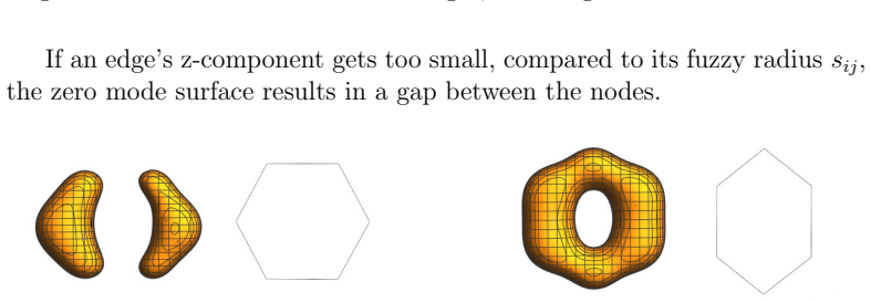
The central claim rests on a narrowly hand-tuned Trefoil graph: the edge radii, edge directions, and the balance between vertex count and edge length must be chosen so that the zero-mode surface neither self-intersects nor separates, and the paper reports that too few vertices or longer edges destroy the knot shape.
Editorial extensions
If this is right
- A nonsymmetric, topologically nontrivial surface such as a Trefoil knot can be captured by zero-mode surfaces, extending fuzzy geometry beyond spheres and tori.
- Edge direction acts as a topology control: reversing an edge can change the zero-mode surface from a sphere to an hourglass, so the encoding is not invariant under edge reversal.
- Interpolating the matrices of a fuzzy cylinder and a fuzzy torus yields a continuous change of the zero-mode surface, with a topology change from genus 0 to genus 1 occurring when the deformed ends touch at a single point.
- Zero-curvature gauge-field deformations can alter the graph data (radii, node ordering) while leaving the zero-mode surface unchanged, separating geometric shape from matrix data.
- The graph-to-matrix workflow can in principle be applied to more complex knots and links, limited mainly by the growth of the determinant polynomial with matrix size.
Reading between the lines
- The determinant polynomial of the Trefoil knot is itself an algebraic surface invariant; extracting invariants such as its singular locus or braid structure could yield knot data (for instance the Alexander polynomial), a testable extension the authors raise only as a question.
- The narrow stability window in vertex count and edge length suggests the construction behaves like a numerical discretization of an embedded curve: for fixed matrix size there is a critical edge-length-to-radius ratio, so the method may be better described as a discretization scheme than a universal quantization.
- Edge orientation looks like a discrete gauge degree of freedom; scanning all edge-direction choices for a fixed graph could connect zero-mode surfaces to framings or Seifert surfaces of the knot.
- Because block-diagonal matrices split determinants into factors, complex fuzzy surfaces could be assembled from simpler fuzzy pieces; building the Trefoil from overlapping fuzzy spheres or cylinders would give a tunable way to test stability.
Editorial analysis
A structured set of objections, weighed in public.
Referee Report
Summary. The paper presents a workflow for constructing fuzzy spaces from 3D graphs: a Python script extracts graph data from Blender into Hermitian matrices X, Y, Z, and a Mathematica notebook plots the zero-mode surface defined by det(Σ_a γ^a (X^a - x^a)) = 0. The central claimed result is that a hand-built 30-node Trefoil-shaped graph yields a two-dimensional Trefoil knot as a zero-mode surface (Section 3.1, Figure 8). Additional examples illustrate transitions from cylinder to torus (Section 4.1), separation of zero-manifolds (Section 4.2), and gauge-field deformations (Section 4.3). The authors state in the conclusions that the commutator and explicit matrix forms are not crucial and that the zero-mode polynomials deserve further analysis.
Significance. If the Trefoil claim were rigorously established, it would provide a concrete example of a nontrivial knot realized as a fuzzy zero-mode surface, potentially connecting matrix-model membranes with knot theory. The paper's strengths include exact determinant computations for small examples (e.g., the fuzzy sphere in Section 2.1, Eq. (17)), a clear demonstration of how edge direction affects the zero-mode surface, and parameter-dependent transitions that are useful for visualization. However, the headline result is currently unsupported by topological data, explicit matrices, or a classical limit, so the significance is sharply conditional on whether the missing evidence can be supplied.
major comments (4)
- [§3.1, Figure 8] The identification of the zero-mode surface as a Trefoil knot is based only on a rendered contour plot; no explicit 30×30 matrices X, Y, Z, no polynomial P(x, y, z), and no topological invariant (e.g., Alexander polynomial, knot group, or an ambient-isotopy certificate) are provided in the manuscript. Since the real zero set of a determinant polynomial can contain multiple components, self-intersections, or higher-dimensional singular strata, the image alone does not establish that the surface is a single connected 2-manifold in the Trefoil ambient-isotopy class.
- [§3.1, Figures 6-7] The edge radii s_x, s_y and edge directions for the 30-node Trefoil graph are not documented numerically; the text only says that edges had to be kept shorter than the distance between separate parts of the mesh and that too few vertices cause the surface to separate. This makes the construction irreproducible from the manuscript and leaves the claimed Trefoil surface dependent on undocumented manual tuning that may not be robust to reasonable variations in the input graph.
- [§5] The authors state that 'the commutator or the explicit form of the matrices is not crucial' and that the polynomials 'deserve further analysis.' These statements acknowledge the absence of the core data needed to verify the central claim, which is precisely the polynomial zero locus. Moreover, no sequence of approximating matrices with a classical limit (N → ∞) is given, so the term 'quantization' is not justified in the standard fuzzy-geometry sense used in [10] and [15].
- [§3.1] Because the graph was explicitly shaped like a Trefoil knot in Blender, the resemblance of the zero-mode surface to a Trefoil is partly by construction rather than an independent prediction. A stronger demonstration would include a stability test under random perturbations of node positions or a comparison of the determinant polynomial with the defining equations of a standard Trefoil parametrization, showing that the topological type is not an artifact of the specific hand-tuned graph.
minor comments (6)
- [§2.1, Eq. (20)] The rule Y_ji = -s_yij makes Y Hermitian only because s_yij is chosen purely imaginary; this should be stated explicitly to avoid confusion for readers who might otherwise assume real edge labels.
- [§4.1, Eq. (23) and text] The convex-combination formula is written inconsistently as X^a(p) = (p - 1) X^a_C + p X^a_T while the operator is defined as H(p) = (1 - p) H_C + p H_T; the sign convention should be harmonized.
- [§4.3, Eq. (32)] The dots in the matrices are explained as 'negative transposed upper triangular matrix entries,' but the explanation is ambiguous; a full expression or a clearer notational convention would improve readability.
- [§5] The sentence 'An alternative workflow is presented, using Blender's volume shading...' appears twice in the conclusions; the duplication should be removed.
- [§6, references [17]-[18]] The scripts and notebooks are linked to Google Drive folders; for archival stability, these should be included as supplementary material or deposited in a permanent repository with versioned identifiers.
- [§3.1] The claim that 30 nodes is the fewest that capture the Trefoil geometry is not supported by a systematic search description or quantitative error metrics; please clarify the criteria used to decide that fewer vertices are insufficient.
Circularity Check
The fuzzy Trefoil 'result' is the input graph re-covered by construction: the graph is modeled as a Trefoil and the zero-mode surface is tuned to match it.
-
fitted input called prediction
[Section 3.1 (Fuzzy Trefoil knot), Figures 6-8; see also Eq. (18) and the Abstract.]
"With the above presented method, we construct a Trefoil knot as 3D-graph and plot a zero mode surface from it. The plot represents a two dimensional Trefoil knot embedded in R3. ... The edges had to be kept shorter than the distance between the separate parts of the mesh. Otherwise, the parts would intersect. If fewer vertices are used to form the knot, the edge lengths increase until the fuzzy surface separates into distinct parts."
By Eq. (18), the zero-mode surface is the determinant zero set det(sum_a gamma^a (X^a - x^a 1)) = 0, a deterministic function of matrices X^a, Y, Z. Those matrices are read off from the graph through Eqs. (19)-(21): diagonals are node coordinates and off-diagonal entries are edge radii. The graph was explicitly modeled in Blender as a Trefoil knot, and Section 3.1 describes tuning the number of vertices and edge lengths/radii until the rendered surface neither intersects nor separates. Hence the announced 'quantization of a two-dimensional Trefoil knot' is not an independent prediction of the method; it is the same Trefoil shape that was put into the graph, recovered as the determinant locus because the parameters were adjusted to make that happen.
full rationale
The underlying map from graphs to zero-mode surfaces (Section 2) is exact and not itself circular: once the matrices are given, the determinant polynomial and its zero set are well-defined outputs. The circularity is in the presentation of the headline example: a graph already shaped like a Trefoil, with edge radii and vertex counts hand-tuned so that the determinant surface does not self-intersect or separate, is then reported as a 'result' showing quantization of a Trefoil knot. This is a fitted input called a result rather than an independent derivation. The cylinder-to-torus and separation examples are likewise constructed by choosing matrices that interpolate between known shapes, but those are illustrative demonstrations rather than claimed predictions. The paper also omits explicit matrices and a topological certificate for the Trefoil, which weakens the claim further, but that is an evidentiary gap rather than an additional circular step. Overall, the central Trefoil claim reduces by construction to the hand-built graph, while the general method retains independent content.
Assumptions & free parameters
free parameters (3)
- Trefoil node count =
30
- Trefoil edge radii s_x, s_y =
Not printed; stored in notebook
- Gauge deformation coefficients A^a_alpha =
Specific ad hoc values used for plots
assumptions (3)
- domain assumption The determinant equation det(sum gamma^a (X^a - x^a 1)) = 0 defines the zero-mode surface that represents the fuzzy space.
- domain assumption The graph-to-matrix encoding of Section 2.1 (diagonal node coordinates, off-diagonal edge labels with X_ij = s_x, Y_ij = s_y, Y_ji = -s_y) is valid for arbitrary directed graphs.
- ad hoc to paper The real locus of the plotted algebraic surface is visually identified with a Trefoil knot.
Cite this review
Pith. "Pith review of Fuzzy-Space Engineering." pith.science (2026). https://pith.science/paper/UJCCPMDF
@misc{pith2026241216011,
  author       = {Pith},
  title        = {Pith review of: Fuzzy-Space Engineering},
  year         = {2026},
  howpublished = {\url{https://pith.science/paper/UJCCPMDF}},
  note         = {Machine review of arXiv:2412.16011}
}
read the original abstract
The techniques developed for matrix models and fuzzy geometry are powerful tools for representing strings and membranes in quantum physics. We study the representation of fuzzy surfaces using these techniques. This involves constructing graphs and writing their coordinates and connectivity into matrices. To construct arbitrary graphs and quickly change them, we use 3D software. A script generates the three matrices from the graphs. These matrices are then processed in Wolfram Mathematica to calculate the zero modes of the Dirac operator. Our first result shows the quantization of a two-dimensional Trefoil knot. Additional examples illustrate various properties and behaviors of this process. This helps us to gain a deeper understanding of fuzzy spaces and zero-mode surfaces. This work contributes to advancing the understanding of visualization aspects in fuzzy geometry.
Figures


Figures from the paper (12 more)



Reference graph
Works this paper leans on
-
[10]
The fuzzy space construction kit,
A. Sykora, “The fuzzy space construction kit,” [arXiv:1610.01504 [hep-th]]. https://arxiv.org/abs/1610.01504
-
[15]
A new class of fuzzy spaces with classical limit
A. Sykora, “A new class of fuzzy spaces with classical limit,” [arXiv:1709.08886 [hep-th]]. https://arxiv.org/abs/1709.08886
-
[1]
N. Ishibashi, H. Kawai, Y. Kitazawa and A. Tsuchiya, Nucl. Phys. B498, 467- 491 (1997) doi:10.1016/S0550-3213(97)00290-3 [arXiv:hep-th/9612115 [hep- th]]. https://arxiv.org/abs/hep-th/9612115
arXiv 1997
- [2]
-
[3]
Noncommutative Geometry and Ma- trix Theory: Compactification on Tori,
A. Connes, M.R. Douglas, A. Schwarz “Noncommutative Geometry and Ma- trix Theory: Compactification on Tori,” (1998). [arXiv:9711162 [hep-th]] https://arxiv.org/abs/hep-th/9711162
arXiv 1998
-
[4]
W. Taylor, Rev. Mod. Phys. 73 (2001), 419-462 doi:10.1103/RevModPhys.73.419 [arXiv:hep-th/0101126 [hep-th]]. https://arxiv.org/abs/hep-th/0101126
arXiv 2001
-
[5]
B. Ydri, Review of M(atrix)-Theory, Type IIB Matrix Model and Matrix String Theory,” [arXiv:1708.00734 [hep-th]]. https://arxiv.org/abs/1708. 00734
-
[6]
Matrix embeddings on flat $R^3$ and the geometry of membranes
D. Berenstein and E. Dzienkowski, “Matrix embeddings on flat R3 and the geometry of membranes,” Phys. Rev. D 86, 086001 (2012) doi:10.1103/PhysRevD.86.086001 [arXiv:1204.2788 [hep-th]]. https: //arxiv.org/abs/1204.2788
work page Pith review arXiv 2012
Show all 18 references
-
[7]
Matrix Geometry and Coherent States,
G. Ishiki, “Matrix Geometry and Coherent States,” Phys. Rev. D 92 (2015) no.4, 046009 doi:10.1103/PhysRevD.92.046009 [arXiv:1503.01230 [hep-th]]. https://arxiv.org/abs/1503.01230
2015 arXiv
-
[8]
Coherent states for arbitrary Lie group,
A. M. Perelomov, “Coherent states for arbitrary Lie group,” Comm. Math. Phys. 26, 222-236 (1972)
1972
-
[9]
M. H. de Badyn, J. L. Karczmarek, P. Sabella-Garnier and K. H. C. Yeh, JHEP 11, 089 (2015) doi:10.1007/JHEP11(2015)089 [arXiv:1506.02035 [hep- th]]. https://arxiv.org/abs/1506.02035
2015 arXiv
-
[11]
Measuring finite Quantum Ge- ometries via Quasi-Coherent States,
L. Schneiderbauer and H. C. Steinacker, “Measuring finite Quantum Ge- ometries via Quasi-Coherent States,” J. Phys. A 49 (2016) no.28, 285301 doi:10.1088/1751-8113/49/28/285301 [arXiv:1601.08007 [hep-th]]. https:// arxiv.org/abs/1601.08007
2016 arXiv
-
[12]
Quantum Theory of a Massless Relativistic Surface and a Two- Dimensional Bound State Problem,
J. R. Hoppe, “Quantum Theory of a Massless Relativistic Surface and a Two- Dimensional Bound State Problem,” PhD thesis, Massachusetts Institute of Technology, 1982
1982
-
[13]
The Fuzzy Sphere,
J. Madore, “The Fuzzy Sphere,” Class. Quant. Grav.9, 69 (1992)
1992
-
[14]
Shimada, Nucl
H. Shimada, Nucl. Phys. B 685, 297-320 (2004) doi:10.1016/j.nuclphysb.2004.02.017 [arXiv:hep-th/0307058 [hep-th]]. https://arxiv.org/abs/hep-th/0307058 24
2004 arXiv
-
[16]
Python script: Node expressions
R. Sedman, “Python script: Node expressions”. https://blendermarket. com/products/node-expressions
-
[17]
Python script: fuzzy engineering
R. Schweiger, “Python script: fuzzy engineering”. https://drive.google. com/file/d/1HgPpSPk5PAgKs8xpG6nMRKobC4A4dfB1/view?usp=sharing
-
[18]
Mathematica notebooks repository
R. Schweiger, P. Schreivogl “Mathematica notebooks repository”. https://drive.google.com/drive/folders/ 1O1t1o4CVY0-RafOXq0y3rycLowuyybLp?usp=sharing 25
Reviewed August 11, 2026 · model on record in the stance chip above.
Discussion (0). Continue with ORCID to comment.