REVIEW 1 major objections 5 minor 1 cited by
Adaptive Conformal Inference by Betting
T0 review · 1 major / 5 minor · reviewed 2026-08-11 · deepseek-v4-flash
Pith's one-line read The paper claims that a coin-betting update for conformal prediction intervals can remove learning-rate tuning entirely while still achieving the nominal long-term miscoverage rate, and that the resulting parameter-free predictor is…
desk verdict A genuinely useful parameter-free alternative to tuned OGD in adaptive conformal inference, but the long-term coverage theorem has a circular step in Appendix B and is not proven as written. read the letter →
The pith
A machine-rendered reading of the paper's core claim, the machinery that carries it, and where it could break.
The reading
What carries the argument
The central object is the coin-betting view of online convex optimization, specialized to pinball-loss quantile estimation. In Algorithm 1, the coin outcome is c_t = -g_t, where g_t is a subgradient of the pinball loss at the current radius; the gambler bets a fraction λ_{t+1} of current wealth W_t, so the next radius is s_{t+1} = λ_{t+1} W_t. The KT estimator provides the update λ_{t+1} = (t/(t+1))λ_t - g_t/(t+1). This machinery does two jobs: it yields a sub-linear regret bound with no tuned constants, and it converts any persistent deviation of the miscoverage rate from α into exponentially growing radii, which is the engine of Theorem 2.1.
What would settle it
Simulate Algorithm 1 on a long stream of bounded scores chosen adversarially from {0,D} while recording the running miscoverage; if any such stream yields a limiting miscoverage different from α, Theorem 2.1 is false. As a first check, verify whether |s_t| ever exceeds 3D+1 on such a stream.
Extended reading notes
Core claim
The central claim is that the price of learning-rate tuning can be eliminated entirely: a conformal predictor whose radii are updated by the Krichevsky-Trofimov betting rule (Algorithm 1 in the paper) satisfies the long-term coverage guarantee for any data stream whose nonconformity scores are bounded by an unknown constant D, with no user-set parameters. The proof builds a bridge between quantile estimation and betting: the coin outcomes are the negated subgradients of the pinball loss, the gambler's wealth is W_t = 1 - Σ g_i s_i, and the radius at time t+1 is s_{t+1} = λ_{t+1} W_t with λ updated by the KT rule. The argument shows that if the average miscoverage failed to converge to α, the wealth lower bound for the KT bettor would force the radii |s_t| to grow without bound, contradicting a claimed boundedness of the iterates; the paper concludes that coverage must converge. The claim is stated for α ∈ (0, 1/2) and relies on the scores lying in [0, D].
Load-bearing premise
The guarantee rests on an unproven claim that the prediction intervals stay within about three times the largest observed error, and the paper's proof of that claim assumes the intervals never exceed the largest observed error in the first place.
Editorial extensions
If this is right
- If Theorem 2.1 stands, adaptive conformal inference can be run on arbitrary data streams with bounded scores and no learning-rate tuning while still converging to the target miscoverage frequency.
- The same betting update can be run independently for each horizon in multi-step forecasting, so per-horizon intervals inherit the guarantee without extra tuning.
- The method applies to any family of nested prediction sets parameterized by a single radius, including quantile-regression interval recalibration, not just symmetric absolute-error bands.
- The sub-linear pinball-loss regret bound rules out trivial predictors that satisfy coverage by alternating between empty and full sets.
- A practitioner loses at most a small finite-sample coverage gap relative to tuned gradient methods, while gaining invariance to the scale of residuals.
Reading between the lines
- If the circular boundedness step in Appendix B is repaired or replaced, the same betting mechanism could plausibly extend to non-bounded or heavy-tailed scores through clipping or truncation, a direction the paper does not analyze.
- The coverage guarantee is asymptotic; a finite-sample or non-asymptotic version, such as a probability bound on miscoverage deviation after T steps, is a natural next step that the paper leaves implicit.
- Because the KT update carries no scale information at all, a direct comparison against alternative parameter-free or scale-free online optimizers on adversarially shifted streams would sharpen the claim that no tuning is needed.
Signed reviews
Editorial analysis
A structured set of objections, weighed in public.
Referee Report
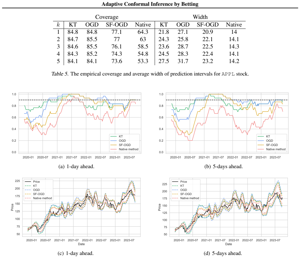
Summary. This paper proposes a parameter-free adaptive conformal inference method based on coin-betting online convex optimization, specifically a Krichevsky-Trofimov (KT) betting strategy (with an Online Newton Step variant in the appendix). The principal theoretical claim (Theorem 2.1) is that, for bounded nonconformity scores with S_t ∈ [0, D], the KT-based algorithm achieves the long-term miscoverage guarantee (1) without any tuning. The paper also provides regret bounds, discusses the necessity of bounded scores, and presents simulations on changepoint, electricity demand, and stock price data comparing the betting approach against tuned OGD/SF-OGD baselines.
Significance. The contribution is potentially valuable: if the coverage guarantee is established, the method is a parameter-free adaptive conformal predictor that avoids learning-rate tuning, a recognized weakness of existing OGD-based methods. The paper gives an explicit, simple algorithm and a regret statement, and the empirical study is broad, covering simulated changepoint data, electricity demand, and multi-horizon stock price forecasting. The KT variant has no fitted constants, which is a strength. However, the central theorem's proof contains a gap in the boundedness step, so the main coverage guarantee is not yet proven as written; this limits the significance of the theoretical contribution and should be addressed before the results can be relied upon.
major comments (1)
- [Appendix B, Step 2 (Eq. (8) and following display)] The proof of the uniform bound |s_t| ≤ 3D+1 is circular. The displayed estimate immediately after Eq. (8) bounds the right-hand side by (D + 1 + D(t−1) + 1 + Dt)/(t+1), where the term D for |s_t| and the term D(t−1) for |Σ_{i=1}^{t−1} g_i s_i| both assume that the iterates before time t satisfy |s_i| ≤ D. That is exactly the conclusion being proved. Step 1 only shows local directional behavior (a radius above D is followed by a decrease, and a nonnegative radius followed by a negative one is followed by a positive one); it does not bound the magnitude of an excursion above D or below 0, and the assertion that the decrease 'repeats until' the radius becomes ≤ D is not established. Consequently, the boundedness conclusion |s_t| ≤ 3D+1 is unsupported, and Step 3's contradiction depends on that bound to rule out the unbounded iterates that the KT wealth lower bound would produce when (1) fails. The coverage guarantee is therefore not proven as written.
minor comments (5)
- [Section 3 and Impact Statement] The text says code is provided as a supplement, but no URL or repository identifier appears in the manuscript; please add a working link or a detailed availability statement.
- [Figures 1–5 and Tables 1–7] The experiments report averages over 200–250 seeds or over a test period, but no standard errors, confidence intervals, or seed-level variability are given; several reported differences (e.g., KT versus OGD coverage around 0.9–1 percentage point) are small enough that variability information is needed to assess them.
- [Figure 5 caption] The caption contains a duplicated phrase 'versions of versions of online gradient descent'; also the footnote marker in Section 3 appears as 'Figure 6¹', which is confusing.
- [Equation (6)] The regret bound introduces a universal constant C without specifying its value or provenance; please state whether C is explicit and how it enters the proof of Theorem 2.1.
- [Appendix A, Algorithm 2] Algorithm 2 is presented as part of the proposed approach and is evaluated in the experiments, but no coverage or regret guarantee is claimed for it; please add a sentence clarifying that the theoretical results apply only to the KT-based Algorithm 1.
Circularity Check
The central coverage theorem is unproved because its key boundedness step is circular: Appendix B Step 2 derives |s_t| <= 3D+1 by assuming |s_t| <= D when bounding |s_{t+1} - s_t|, and Step 3's KT-wealth contradiction depends on that assumed bound.
-
other
[Appendix B, Step 2 of the proof of Theorem 2.1, the estimate following Eq. (8) and the conclusion that the KT iterates are bounded.]
"From (8) and (7), it follows that: |st+1 − st| ≤ 1/(t+1)(D + 1 +D(t − 1) + 1 +Dt) ≤ 2D + 1. Combining that with the fact that s1 = 0 ∈ [0, D] and the result in step 1, we conclude that the iterates of the KT algorithm are bounded: |st| ≤3D + 1."
After Eq. (8), |s_{t+1} − s_t| is bounded by (D + 1 + D(t−1) + 1 + Dt)/(t+1). The leading D and the trailing Dt come from replacing |s_t| and |s_t Σ_{i≤t} g_i| by D and Dt respectively, i.e., from assuming every iterate so far (in particular s_t) lies in [−D, D]. That is precisely the boundedness being proved; the conclusion |s_t| ≤ 3D+1 is a trivial consequence of assuming |s_t| ≤ D and does not follow from |s_{t+1} − s_t| ≤ 2D+1 with s_1 = 0 alone. Step 3's contradiction — KT wealth exploding when (1) fails — requires this uniform bound to rule out unbounded iterates, so Theorem 2.1's coverage claim is supported only by assuming the boundedness it must derive. This is a proof-internal petitio principii at a load-bearing point.
full rationale
Score 6, partial circularity of the central proof rather than a fit-based reduction. The main theoretical claim is Theorem 2.1: Algorithm 1 achieves long-term coverage (1) under bounded nonconformity scores S_t ∈ [0,D]. The proof chain requires Step 2 to establish uniform boundedness of the KT iterates (|s_t| ≤ 3D+1) so that Step 3's KT wealth lower bound yields a contradiction when (1) fails. Step 2's estimate after Eq. (8) bounds |s_{t+1} − s_t| by substituting D for |s_t| and Dt for |s_t Σ g_i|, which assumes precisely the boundedness under investigation; the conclusion is weaker than the assumption used to derive it, so no independent bound is established. Step 3's contradiction thereby rests on an assumed uniform bound, and Theorem 2.1 is unproved as written. This is distinguishable from fitted-input circularity: no parameter is fitted to data, no prediction is a renamed fit, and the KT/ONS wealth and regret bounds are imported from external work (Orabona & Pál 2016; Cutkosky & Orabona 2018), not from author-authored results. The only self-citation (Podkopaev & Ramdas 2021) appears in related-work context and is not load-bearing, and the empirical comparisons are self-contained. I therefore flag the circular Step-2 boundedness argument as the single load-bearing circular step while noting that an independent boundedness proof could repair the theorem.
Assumptions & free parameters
assumptions (5)
- domain assumption Bounded nonconformity scores: S_t in [0,D] for all t.
- domain assumption Target miscoverage alpha in (0,1/2).
- standard math KT wealth lower bound W_t >= (1/(K sqrt(t))) exp(t/4 (average g)^2).
- standard math Wealth never becomes negative and subgradients satisfy |g_t| <= 1.
- standard math Regret bound (6) for KT betting.
Cite this review
Pith. "Pith review of Adaptive Conformal Inference by Betting." pith.science (2026). https://pith.science/paper/JBESRVLL
@misc{pith2026241219318,
  author       = {Pith},
  title        = {Pith review of: Adaptive Conformal Inference by Betting},
  year         = {2026},
  howpublished = {\url{https://pith.science/paper/JBESRVLL}},
  note         = {Machine review of arXiv:2412.19318}
}
read the original abstract
Conformal prediction is a valuable tool for quantifying predictive uncertainty of machine learning models. However, its applicability relies on the assumption of data exchangeability, a condition which is often not met in real-world scenarios. In this paper, we consider the problem of adaptive conformal inference without any assumptions about the data generating process. Existing approaches for adaptive conformal inference are based on optimizing the pinball loss using variants of online gradient descent. A notable shortcoming of such approaches is in their explicit dependence on and sensitivity to the choice of the learning rates. In this paper, we propose a different approach for adaptive conformal inference that leverages parameter-free online convex optimization techniques. We prove that our method controls long-term miscoverage frequency at a nominal level and demonstrate its convincing empirical performance without any need of performing cumbersome parameter tuning.
Figures


Figures from the paper (14 more)




Forward citations
Cited by 1 Pith paper
-
CUSUM-Shaped Inference-Time Monitoring and Targeted Re-Decoding for Quantized Small Language Model Reasoning
A monitoring-guided rollback controller produced a small and statistically uncertain accuracy gain on first-seen MATH-500 problems, and a larger exploratory gain on a historical-coverage set contaminated by manual thr...
Reference graph
Works this paper leans on
-
[1]
write newline
" write newline "" before.all 'output.state := FUNCTION n.dashify 't := "" t empty not t #1 #1 substring "-" = t #1 #2 substring "--" = not "--" * t #2 global.max substring 't := t #1 #1 substring "-" = "-" * t #2 global.max substring 't := while if t #1 #1 substring * t #2 global.max substring 't := if while FUNCTION format.date year duplicate empty "emp...
-
[2]
Angelopoulos, A., Cand \`e s, E. J., and Tibshirani, R. J. Conformal pid control for time series prediction. In Advances in Neural Information Processing Systems, 2023
work page 2023
-
[3]
Angelopoulos, A. N. and Bates, S. Conformal prediction: A gentle introduction. Foundations and Trends in Machine Learning , 2023
work page 2023
-
[4]
Barber, R. F., Cand \`e s, E. J., Ramdas, A., and Tibshirani, R. J. Predictive inference with the jackknife+ . The Annals of Statistics, 2021
work page 2021
-
[5]
Barber, R. F., Cand \`e s, E. J., Ramdas, A., and Tibshirani, R. J. Conformal prediction beyond exchangeability . The Annals of Statistics, 2023
work page 2023
-
[6]
Improved online conformal prediction via strongly adaptive online learning
Bhatnagar, A., Wang, H., Xiong, C., and Bai, Y. Improved online conformal prediction via strongly adaptive online learning. In International Conference on Machine Learning, 2023
work page 2023
-
[7]
Cand \`e s, E. J., Lei, L., and Ren, Z. Conformalized survival analysis . Journal of the Royal Statistical Society Series B: Statistical Methodology, 2023
work page 2023
-
[8]
Cesa-Bianchi, N. and Lugosi, G. Prediction, learning, and games. Cambridge University Press, 2006
work page 2006
Show all 30 references
-
[9]
Exact and robust conformal inference methods for predictive machine learning with dependent data
Chernozhukov, V., W\" u thrich, K., and Yinchu, Z. Exact and robust conformal inference methods for predictive machine learning with dependent data. In Conference On Learning Theory, 2018
2018
-
[10]
and Orabona, F
Cutkosky, A. and Orabona, F. Black-box reductions for parameter-free online learning in banach spaces. In Conference On Learning Theory, 2018
2018
-
[11]
N., Listgarten, J., and Jordan, M
Fannjiang, C., Bates, S., Angelopoulos, A. N., Listgarten, J., and Jordan, M. I. Conformal prediction under feedback covariate shift for biomolecular design. Proceedings of the National Academy of Sciences, 2022
2022
-
[12]
and Cand \`e s, E
Gibbs, I. and Cand \`e s, E. J. Adaptive conformal inference under distribution shift. In Advances in Neural Information Processing Systems, 2021
2021
-
[13]
and Cand \`e s, E
Gibbs, I. and Cand \`e s, E. J. Conformal inference for online prediction with arbitrary distribution shifts. In arXiv preprint: 2305.12616, 2022
2022 arXiv
-
[14]
K., and Ramdas, A
Gupta, C., Kuchibhotla, A. K., and Ramdas, A. Nested conformal prediction and quantile out-of-bag ensemble methods. Pattern Recognition, 2022
2022
-
[15]
Splice-2 comparative evaluation: Electricity pricing
Harries, M. Splice-2 comparative evaluation: Electricity pricing. Technical report, University of New South Wales, 1999
1999
-
[16]
Logarithmic regret algorithms for online convex optimization
Hazan, E., Agarwal, A., and Kale, S. Logarithmic regret algorithms for online convex optimization. Machine Learning, 2007
2007
-
[17]
Kelly, J. L. A new interpretation of information rate. IRE Transactions on Information Theory, 1956
1956
-
[18]
and Trofimov, V
Krichevsky, R. and Trofimov, V. The performance of universal encoding. IEEE Transactions on Information Theory, 1981
1981
-
[19]
and Cand \`e s, E
Lei, L. and Cand \`e s, E. J. Conformal inference of counterfactuals and individual treatment effects. Journal of the Royal Statistical Society Series B: Statistical Methodology, 2021
2021
-
[20]
and Pál, D
Orabona, F. and Pál, D. Coin betting and parameter-free online learning. In Advances in Neural Information Processing Systems, 2016
2016
-
[21]
and Pál, D
Orabona, F. and Pál, D. Scale-free online learning. Theoretical Computer Science, 2018
2018
-
[22]
and Ramdas, A
Podkopaev, A. and Ramdas, A. Distribution-free uncertainty quantification for classification under label shift. In Uncertainty in Artificial Intelligence, 2021
2021
-
[23]
Conformalized quantile regression
Romano, Y., Patterson, E., and Cand \`e s, E. Conformalized quantile regression. In Advances in Neural Information Processing Systems, 2019
2019
-
[24]
Alaa, A., and van der Schaar, M
Stankeviciute, K., M. Alaa, A., and van der Schaar, M. Conformal time-series forecasting. In Advances in Neural Information Processing Systems, 2021
2021
-
[25]
Taylor, S. J. and Letham, B. Forecasting at Scale . The American Statistician, 2018
2018
-
[26]
J., Barber, R
Tibshirani, R. J., Barber, R. F., Candes, E., and Ramdas, A. Conformal prediction under covariate shift. In Advances in Neural Information Processing Systems, 2019
2019
-
[27]
Algorithmic Learning in a Random World
Vovk, V., Gammerman, A., and Shafer, G. Algorithmic Learning in a Random World. Springer-Verlag, 2005
2005
-
[28]
and Xie, Y
Xu, C. and Xie, Y. Conformal prediction interval for dynamic time-series. In International Conference on Machine Learning, 2021
2021
-
[29]
and Xie, Y
Xu, C. and Xie, Y. Sequential predictive conformal inference for time series. In International Conference on Machine Learning, 2023
2023
-
[30]
Adaptive conformal predictions for time series
Zaffran, M., Feron, O., Goude, Y., Josse, J., and Dieuleveut, A. Adaptive conformal predictions for time series. In International Conference on Machine Learning, 2022
2022
Reviewed August 11, 2026 · model on record in the stance chip above.
Discussion (0). Continue with ORCID to comment.