REVIEW 4 major objections 7 minor 1 cited by
Application of normalizing flows to nuclear many-body perturbation theory
T0 review · 4 major / 7 minor · reviewed 2026-08-10 · deepseek-v4-flash
Pith's one-line read Normalizing flows cut Monte Carlo integration error in nuclear many-body calculations by an order of magnitude, even for pole-divergent response integrals.
desk verdict A solid methods extension of normalizing-flow importance sampling to principal-value response integrals, but the order-of-magnitude advantage over VEGAS needs a specified baseline before it can be trusted. read the letter →
The pith
A machine-rendered reading of the paper's core claim, the machinery that carries it, and where it could break.
The reading
What carries the argument
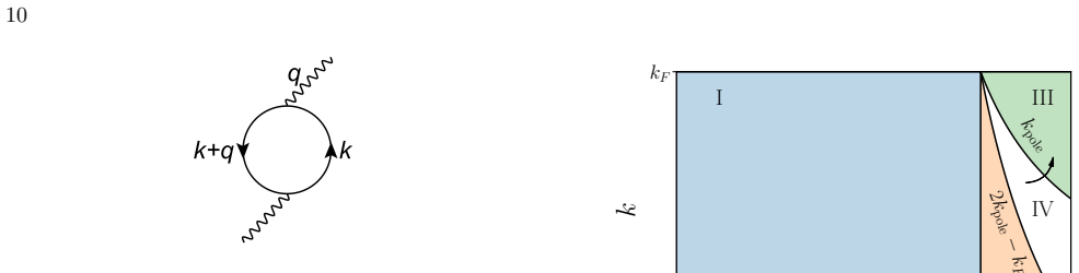
The engine is a normalizing flow built from alternating coupling layers of rational quadratic splines: each layer leaves some coordinates fixed while neural networks generate the spline parameters that transform the others, so the Jacobian stays triangular and the full map stays invertible. Training minimizes a divergence between the transformed density and the normalized absolute integrand $|\psi(\vec x)|/\tilde I$, and the same samples then estimate the integral by the importance weight $\psi(\vec x)/p(\vec x)$. For the response function, the pole line $k_{\rm pole}$ from Eq. (39) is handled either by reflection, folding one side of the integrand across the pole so the divergences cancel, or by subtraction, removing the singular piece and integrating the logarithm analytically; each resulting finite integral is assigned its own flow.
What would settle it
Run VEGAS on the same two integrals with the same total computational budget, scanning batch size and adaptation settings, and compare true errors against converged Gaussian-quadrature references; if a tuned VEGAS closes the factor-of-ten gap, the central performance claim collapses.
Extended reading notes
Core claim
The central claim is that normalizing flows provide a practical, high-accuracy Monte Carlo sampling tool for the integrands that appear in nuclear matter perturbation theory, including irregular integrands with a pole line. For the seven-dimensional second-order contribution $\Omega^{(2)}$ to the grand canonical potential and for the zeroth-order density-density response function $\chi(q,\omega)$, the authors compare the batch relative error of flow-based importance sampling with VEGAS and find the flow errors are at least an order of magnitude smaller after training. They show that both the reflection and subtraction strategies for Cauchy principal value integrals can be implemented with flows, with reflection giving a moderate efficiency gain. They also demonstrate model transfer: a flow trained at one density and temperature, or at one momentum and energy transfer $(q,\omega)$, can be reused at nearby values, and the flow adapts when the nuclear potential is replaced by a chiral pion-exchange interaction.
Load-bearing premise
The order-of-magnitude improvement over VEGAS assumes the VEGAS baseline was given a fair and reasonably optimized configuration, but the paper does not report VEGAS's batch size, adaptation schedule, or tuning effort.
Editorial extensions
If this is right
- The second-order grand canonical potential and the zeroth-order density response function can be integrated with roughly an order of magnitude smaller batch uncertainty than VEGAS at the same sample count.
- A flow trained at one density, temperature, and momentum/energy transfer can be transferred to nearby values with little retraining, which is what a full astrophysical tabulation requires.
- Trained flows remain effective when the interaction is changed to a chiral pion-exchange potential, so uncertainty quantification across nuclear force models becomes more feasible.
- Quasi-random sample generators stabilize training and improve true precision, especially at small batch sizes, and their pointwise variance estimates overstate the actual error.
- Both reflection and subtraction pole treatments work with flows; reflection is modestly more efficient for the cases tested.
Reading between the lines
- The economic case for the method is amortization: training is expensive, but if a single trained model covers a neighborhood of densities, temperatures, and kinematic points, the cost of filling an equation-of-state and response table should fall; a direct wall-clock comparison over a full table would test this.
- The quasi-random generator results suggest that for low-discrepancy samples the per-batch variance estimate is not a reliable uncertainty reporter, so downstream users should quote ensemble spreads over repeated runs rather than the pointwise formula.
- The reflection-versus-subtraction comparison hints that how a principal value pole is decomposed matters more than how the flow learns the remaining integrand; one could test this on other pole geometries, such as curved pole lines, to see whether the ordering persists.
Editorial analysis
A structured set of objections, weighed in public.
Referee Report
Summary. The paper applies normalizing-flow importance sampling to two classes of integrals from nuclear many-body perturbation theory: the seven-dimensional second-order contribution to the finite-temperature grand canonical potential of symmetric nuclear matter (Eq. 32) and the two-dimensional zero-temperature density-density response function, whose real part requires principal-value integration (Eqs. 37-43). The authors compare eight loss functions and four random-number generators (pseudo-random, Sobol, Halton, Lattice), benchmark the EOS integral against converged Gaussian quadrature, and test transferring trained models across temperature, density, momentum/energy transfer, and one nuclear-potential change (scalar-boson exchange to chiral NLO pion exchange). They report that normalizing flows reach batch relative uncertainties at least an order of magnitude below VEGAS, that quasi-random generators improve stability and accuracy, and that point-estimate uncertainties for quasi-random sampling are conservative relative to the spread of independent estimates.
Significance. If the central performance claim survives scrutiny, the paper provides a useful demonstration that learned importance-sampling densities can handle both regular 7D MBPT integrands and singular principal-value integrands, with plausible transferability across thermodynamic and kinematic variables. The strengths are genuine: the EOS results are checked against converged Gaussian quadrature (Figs. 5, 7); the QRNG point-estimate-vs-true-error analysis (Figs. 4-5) is careful and correct in spirit; and treating the pole via both reflection and subtraction is a useful methodological comparison. The main weaknesses are that the VEGAS baseline is not specified, the response-function part lacks an analogous exact benchmark, the normalizing-flow architecture and interaction parameters are unreported, and the zero-fine-tuning transfer claim overstates the protocol actually used. No code is provided. As it stands, the order-of-magnitude claim is plausible but not yet reproducible; the practical 'efficient tabulations' promise is also asserted rather than costed, especially since the response-function examples are two-dimensional integrals where deterministic quadrature would be competitive.
major comments (4)
- [Section III B/III D; Figs. 3, 6, 11, 12] The central 'order of magnitude' claim over VEGAS is not reproducible as presented because the VEGAS configuration is never stated: the manuscript does not report VEGAS's samples per iteration, number of adaptation steps, damping parameter, grid binning, or whether it used the same batch sizes as the normalizing flows (5000 in Fig. 3, 1500 in Fig. 11). The claim in Section III B that 'VEGAS converges to its precision limit within about 100 iterations' is also inconsistent with the accumulation formula (Eqs. (33)-(34)), which for unbiased independent batches would give sigma_t proportional to 1/sqrt(N_iter); the observed plateau is better interpreted as a bias floor, and Fig. 7 confirms that VEGAS's reported uncertainties severely underpredict its true error at low temperature. Please report the VEGAS settings and present the comparison on the basis of true errors (against Gaussian quadrature or analytic results), not only the reported per-batch variance.
- [Section III B/III D; Section IV] The transferability claim is overstated relative to what is actually demonstrated. The conclusion states that a trained model 'can be transferred to nearby phase space points without additional fine training', but Section III B says 'After each new modification, we perform a 100-iteration update for the new models' (Fig. 6), and the Section III D protocol for Fig. 12 runs 100 iterations at the new kinematic point with continued Adam updates, since Section II d updates the neural networks at every iteration. These are warm-started retraining runs, not zero-update transfers. Please correct the wording, and ideally quantify the warm-start benefit by comparing against training from scratch at the target point with the same iteration budget.
- [Section III C/III D; Figs. 11-12] Unlike the EOS calculation, which is validated against converged Gaussian quadrature in Figs. 5 and 7, the response-function results in Figs. 11 and 12 are compared only against VEGAS. Since the conclusion claims an order-of-magnitude reduction of 'errors' for response-function calculations, and since Fig. 7 demonstrates that VEGAS-reported uncertainties can be unreliable, an external accuracy check is needed here. The reduced integral in Eq. (37) is only two-dimensional and the zero-temperature free-gas response has a known analytic (Lindhard) form, so a converged quadrature or analytic benchmark is straightforward to add and would make the response-function claim comparable in rigor to the EOS claim.
- [Section II; Section III A] The numerical setup is under-specified, which prevents reproduction and makes the comparison to VEGAS hard to interpret as a fair, tuned comparison. The text gives no values for the number of coupling layers, the number of spline bins K, the neural-network widths and depths, activation functions, or the learning-rate schedule (only the initial learning rate appears in figure captions). Likewise, the parameters of the scalar-boson interaction (g, m_phi in Eq. (29)) and the cutoff Lambda in Eq. (31) are never given, although all EOS results depend on them. These hyperparameters and coupling parameters, together with the training protocol, should be reported (or the code released) before the quantitative claims can be independently assessed.
minor comments (7)
- [Eq. (4)] Eq. (4) is garbled as printed: the sample-variance estimator should be sigma^2 approximately [1/(N(N-1))] times the sum over i of (psi(x_i)/p(x_i) - mean)^2; the current rendering has lost the 1/N normalization. Please correct.
- [Figure captions] Captions of Figures 3 and 4 state 'n = 0.16 fm^{-1}'; the density unit should be fm^{-3} (Figure 5 is correct).
- [Table I] Table I is difficult to parse and appears to contain typos: the 'rdkl' entry as printed is an unweighted average of log ratios rather than a KL-type divergence, and the 'var' entry as rendered reduces to N^{-1} sum_i (q_i/p_i)^2 - N^{-1} sum_i (q_i/p_i)^2, which vanishes identically; please provide the continuous definitions and the exact implemented estimators.
- [Figure 13] Figure 13 contains placeholder glyphs such as 'fm[box]1' and 'fm[box]2'; these appear to be unresolved LaTeX placeholders and should be replaced with proper units (fm^{-1}, fm^{-2}).
- [Section III D] Section III D, transfer paragraph: the sentence 'After the 100 iterations, new models are generated automatically' is ambiguous; please clarify whether the transferred model continues training at each new point or is re-initialized.
- [Section IV] Section IV: the 'efficient tabulations' motivation should be reconciled with the dimensionality of the examples: the response-function integrals in Eqs. (37) and (45) are two-dimensional after angular reduction, and for such low-dimensional integrals a cost comparison with deterministic quadrature (which the paper itself uses as the benchmark) would strengthen the practical-efficiency claim.
- [Section III B] Section III B, first paragraph: 'Since low temperatures lead to a steep integrands' should read 'a steep integrand' or 'steep integrands'.
Circularity Check
No significant circularity: the flow-based importance sampling is validated against independent Gaussian quadrature, and self-citations are contextual rather than load-bearing.
full rationale
The paper's central numerical claims are not derived from their own conclusions. The normalizing flow is trained to approximate the normalized absolute value of a fixed integrand (Eqs. 22-23), which is the standard importance-sampling target, and the resulting Monte Carlo estimates are benchmarked against well-converged Gaussian quadrature (Figure 5 and the Section III B text) and against direct VEGAS runs, so the reported integral values and error bars rest on an external reference rather than on the trained model itself. Citations to the authors' earlier PRL [47] provide motivation, a previously published integrand formula (Eq. 32), and earlier illustrative precision numbers; they are not used to establish the new transferability or order-of-magnitude claims, which are demonstrated in this paper in Figures 3-4, 6, 11-12 with per-point comparisons and chiral-potential tests. The possible concern that the VEGAS baseline may be undertuned is a comparison-fairness or correctness issue, not a circularity; no step in the manuscript defines a predicted quantity in terms of the fitted model parameters, and no uniqueness theorem is imported from prior work to force the method. Therefore no circular step is present.
Assumptions & free parameters
free parameters (4)
- Normalizing flow hyperparameters =
learning rate 1e-3/1e-4, batch sizes 5000/1500/500/1000, up to 35,000 iterations
- Spline bins and flow layers =
not stated
- VEGAS configuration =
not stated
- Toy model parameters =
not stated in text except Eq. 31; g, m_phi unspecified
assumptions (5)
- standard math Importance sampling estimator Eq. (2) is unbiased and Eq. (4) estimates the variance.
- standard math Rational quadratic spline transformations are invertible and have tractable Jacobians.
- domain assumption The many-body perturbation expansion of the grand canonical potential, Eqs. (26) and (27), is valid for nuclear matter.
- domain assumption The zeroth-order density response function, Eq. (36), can be decomposed using Sokhotski-Plemelj into principal value and delta function parts.
- domain assumption The trained flow distribution closely approximates the normalized absolute integrand.
Cite this review
Pith. "Pith review of Application of normalizing flows to nuclear many-body perturbation theory." pith.science (2026). https://pith.science/paper/T6HAASZB
@misc{pith2026241219777,
  author       = {Pith},
  title        = {Pith review of: Application of normalizing flows to nuclear many-body perturbation theory},
  year         = {2026},
  howpublished = {\url{https://pith.science/paper/T6HAASZB}},
  note         = {Machine review of arXiv:2412.19777}
}
read the original abstract
Many-body perturbation theory provides a powerful framework to study the ground state and thermodynamic properties of nuclear matter as well as associated single-particle potentials and response functions within a systematic order-by-order expansion. However, computational challenges can emerge beyond the lowest orders of perturbation theory, especially when computing both single-particle potentials and response functions, which in general are complex-valued and require Cauchy principal value calculations of high-dimensional integrals. We demonstrate that normalizing flows are suitable for Monte Carlo importance sampling of both regular and irregular functions appearing in nuclear many-body calculations. Normalizing flows are a class of machine learning models that can be used to build and sample from complicated distributions through a bijective mapping from a simple base distribution. Furthermore, a well-trained model for a certain target integrand can be efficiently transferred to calculate related integrals with varying physical conditions. These features can enable more efficient tabulations of nuclear physics inputs to numerical simulations of supernovae and neutron star mergers across varying physical conditions and nuclear force models.
Figures


Figures from the paper (6 more)




Forward citations
Cited by 1 Pith paper
-
PMM-IMSRG emulator for the nuclear equation of state with quantified uncertainties
A parametric-matrix-model emulator reproduces IMSRG nuclear-matter energies with calibrated conformal-prediction error bars, enabling Bayesian fitting of three-nucleon couplings to saturation properties.
Reference graph
Works this paper leans on
-
[1]
H. Shen, H. Toki, K. Oyamatsu, and K. Sumiyoshi, Nucl. Phys. A637, 435 (1998)
work page 1998
- [2]
-
[3]
D. G. Yakovlev, O. Y. Gnedin, M. E. Gusakov, A. D. Kaminker, K. P. Levenfish, and A. Y. Potekhin, Nuclear Physics A Proceedings of the 22nd International Nuclear Physics Conference (Part 2), 752, 590 (2005)
work page 2005
-
[4]
Thermal Effects in Dense Matter Beyond Mean Field Theory
C. Constantinou, S. Lalit, and M. Prakash, Int. J. Mod. Phys. E 26, 1740005 (2017), arXiv:1608.04713 [nucl-th]
work page Pith review arXiv 2017
-
[5]
E. F. Brown, A. Cumming, F. J. Fattoyev, C. J. Horowitz, D. Page, and S. Reddy, Phys. Rev. Lett. 120, 182701 (2018)
2018
- [6]
- [7]
- [8]
Show all 74 references
-
[9]
X. Du, A. W. Steiner, and J. W. Holt, Phys. Rev. C 99, 025803 (2019)
2019
-
[10]
Iwamoto and C
N. Iwamoto and C. J. Pethick, Phys. Rev. D 25, 313 (1982)
1982
-
[11]
R. F. Sawyer, Phys. Rev. C 40, 865 (1989)
1989
-
[12]
nsam- ple
At the beginning of the model transfer, the trained models are used to estimate the density response func- tion for 100 iterations with 1500 samples per iteration at the (q, ω) position where they are trained. After the 100 iterations, new models are generated automatically an...
-
[13]
Reddy, M
S. Reddy, M. Prakash, and J. M. Lattimer, Phys. Rev. C 58, 013009 (1998)
1998
-
[14]
Burrows and R
A. Burrows and R. F. Sawyer, Phys. Rev. C 58, 554 (1998)
1998
-
[15]
Lovato, O
A. Lovato, O. Benhar, S. Gandolfi, and C. Losa, Phys. Rev. C 89, 025804 (2014)
2014
-
[16]
Kotake, T
K. Kotake, T. Takiwaki, T. Fischer, K. Nakamura, and G. Mart ´ ınez-Pinedo, ApJ853, 170 (2018)
2018
-
[17]
C. Shen, U. Lombardo, N. Van Giai, and W. Zuo, Phys. Rev. C 68, 055802 (2003)
2003
-
[18]
Pastore, M
A. Pastore, M. Martini, D. Davesne, J. Navarro, S. Goriely, and N. Chamel, Phys. Rev. C 90, 025804 (2014)
2014
-
[19]
C. J. Horowitz, M. A. P´ erez-Garc ´ ıa, D. K. Berry, and J. Piekarewicz, Phys. Rev. C 72, 035801 (2005)
2005
-
[20]
E. Shin, E. Rrapaj, J. W. Holt, and S. K. Reddy, Phys. Rev. C 109, 015804 (2024)
2024
-
[21]
L. F. Roberts, S. Reddy, and G. Shen, Phys. Rev. C 86, 065803 (2012)
2012
-
[22]
Li, B.-J
B.-A. Li, B.-J. Cai, L.-W. Chen, and J. Xu, Prog. Part. Nucl. Phys. 99, 29–119 (2018)
2018
-
[23]
Rrapaj, J
E. Rrapaj, J. W. Holt, A. Bartl, S. Reddy, and A. Schwenk, Phys. Rev. C 91, 035806 (2015)
2015
-
[24]
Mart ´ ınez-Pinedo, T
G. Mart ´ ınez-Pinedo, T. Fischer, A. Lohs, and L. Huther, Phys. Rev. Lett. 109, 251104 (2012)
2012
-
[25]
Donati, P
P. Donati, P. M. Pizzochero, P. F. Bortignon, and R. A. Broglia, Phys. Rev. Lett. 72, 2835 (1994)
1994
-
[26]
Yasin, S
H. Yasin, S. Sch¨ afer, A. Arcones, and A. Schwenk, Phys. Rev. Lett. 124, 092701 (2020)
2020
-
[27]
Ishizuka, A
C. Ishizuka, A. Ohnishi, K. Tsubakihara, K. Sumiyoshi, and S. Yamada, J. Phys. G: Nucl. Part. Phys.35, 085201 (2008)
2008
- [28]
-
[29]
A. W. Steiner, M. Hempel, and T. Fischer, ApJ 774, 17 (2013)
2013
-
[30]
Oertel, C
M. Oertel, C. Providˆ encia, F. Gulminelli, and A. R. Raduta, J. Phys. G: Nucl. Part. Phys. 42, 075202 (2015)
2015
-
[31]
N. H. Tan, D. T. Loan, D. T. Khoa, and J. Margueron, Phys. Rev. C 93, 035806 (2016)
2016
-
[32]
Hempel and J
M. Hempel and J. Schaffner-Bielich, Nuclear Physics A 837, 210 (2010)
2010
-
[33]
W. Zuo, A. Lejeune, U. Lombardo, and J. F. Mathiot, The European Physical Journal A - Hadrons and Nuclei 14, 469 (2002)
2002
-
[34]
W. Zuo, A. Lejeune, U. Lombardo, and J. F. Mathiot, Nuclear Physics A 706, 418 (2002)
2002
-
[35]
Wellenhofer, J
C. Wellenhofer, J. W. Holt, and N. Kaiser, Phys. Rev. C 93, 055802 (2016)
2016
-
[36]
Wen and J
P. Wen and J. W. Holt, Phys. Rev. C103, 064002 (2021)
2021
-
[37]
Gezerlis, I
A. Gezerlis, I. Tews, E. Epelbaum, S. Gandolfi, K. Hebeler, A. Nogga, and A. Schwenk, Phys. Rev. Lett. 111, 032501 (2013)
2013
-
[38]
Akmal, V
A. Akmal, V. R. Pandharipande, and D. G. Ravenhall, 15 Phys. Rev. C 58, 1804 (1998)
1998
-
[39]
I. Tews, S. Gandolfi, A. Gezerlis, and A. Schwenk, Phys. Rev. C 93, 024305 (2016)
2016
-
[40]
Wlaz lowski, J
G. Wlaz lowski, J. W. Holt, S. Moroz, A. Bulgac, and K. J. Roche, Phys. Rev. Lett. 113, 182503 (2014)
2014
-
[41]
Alexandru, P
A. Alexandru, P. Bedaque, E. Berkowitz, and N. C. Warrington, Phys. Rev. Lett. 126, 132701 (2021)
2021
-
[42]
Buraczynski and A
M. Buraczynski and A. Gezerlis, Phys. Rev. Lett. 116, 152501 (2016)
2016
-
[43]
Holzmann, F
M. Holzmann, F. Calcavecchia, D. M. Ceperley, and V. Olevano, Phys. Rev. Lett. 131, 186501 (2023)
2023
-
[44]
Y.-Z. Ma, Z. Lin, B.-N. Lu, S. Elhatisari, D. Lee, N. Li, U.-G. Meißner, A. W. Steiner, and Q. Wang, Phys. Rev. Lett. 132, 232502 (2024)
2024
-
[45]
Davesne, J
D. Davesne, J. W. Holt, A. Pastore, and J. Navarro, Phys. Rev. C 91, 014323 (2015)
2015
-
[46]
Roggero, F
A. Roggero, F. Pederiva, and G. Orlandini, Phys. Rev. B 88, 094302 (2013)
2013
-
[47]
Brady, P
J. Brady, P. Wen, and J. W. Holt, Phys. Rev. Lett. 127, 062701 (2021)
2021
-
[48]
G. Shen, S. Gandolfi, S. Reddy, and J. Carlson, Phys. Rev. C 87, 025802 (2013)
2013
-
[49]
Tabak and C
E. Tabak and C. Turner, Commun. Pure Appl. Math.66, 145 (2013)
2013
-
[50]
E. G. Tabak and E. Vanden-Eijnden, Commun. Math. Sci. 8, 217 (2010)
2010
-
[51]
Hahn, Comp
T. Hahn, Comp. Phys. Comm. 168, 78 (2005)
2005
-
[52]
Papamakarios, E
G. Papamakarios, E. Nalisnick, D. J. Rezende, S. Mo- hamed, and B. Lakshminarayanan, arXiv:1912.02762 (2019)
2019 arXiv
-
[53]
Drischler, K
C. Drischler, K. Hebeler, and A. Schwenk, Phys. Rev. Lett. 122, 042501 (2019)
2019
- [55]
-
[56]
E. G. Tabak and C. V. Turner, Communications on Pure and Applied Mathematics 66, 145 (2013)
2013
-
[57]
Wirnsberger, A
P. Wirnsberger, A. J. Ballard, G. Papamakarios, S. Aber- crombie, S. Racani` ere, A. Pritzel, D. Jimenez Rezende, and C. Blundell, J. Chem. Phys. 153, 144112 (2020)
2020
-
[58]
G. Yang, X. Huang, Z. Hao, M.-Y. Liu, S. Belongie, and B. Hariharan, arXiv:1906.12320 [cs] (2019), 1906.12320
2019 arXiv
-
[59]
C. Gao, S. H¨ oche, J. Isaacson, C. Krause, and H. Schulz, Phys. Rev. D 101, 076002 (2020)
2020
-
[60]
Kanwar, M
G. Kanwar, M. S. Albergo, D. Boyda, K. Cranmer, D. C. Hackett, S. Racani` ere, D. J. Rezende, and P. E. Shana- han, Phys. Rev. Lett. 125, 121601 (2020)
2020
-
[61]
P. Wen, J. W. Holt, and M. Li, arXiv:2306.13007 (2023)
2023 arXiv
-
[62]
Hajij, G
M. Hajij, G. Zamzmi, R. Paul, and L. Thukar, in 2022 IEEE Healthcare Innovations and Point of Care Tech- nologies (HI-POCT) (2022) pp. 46–49
2022
-
[63]
J. A. GREGORY and R. DELBOURGO, IMA Journal of Numerical Analysis 2, 123 (1982)
1982
-
[64]
Durkan, A
C. Durkan, A. Bekasov, I. Murray, and G. Papamakarios, arXiv:1906.04032 [cs, stat] (2019)
2019 arXiv
-
[65]
Adam: A method for stochastic optimization,
D. P. Kingma and J. Ba, “Adam: A method for stochastic optimization,” (2014)
2014
-
[66]
C. Gao, J. Isaacson, and C. Krause, Machine Learning: Science and Technology 1, 045023 (2020)
2020
-
[67]
Kohn and J
W. Kohn and J. M. Luttinger, Phys. Rev. 118, 41 (1960)
1960
-
[68]
Paszke, S
A. Paszke, S. Gross, F. Massa, A. Lerer, J. Bradbury, G. Chanan, T. Killeen, Z. Lin, N. Gimelshein, L. Antiga, A. Desmaison, A. Kopf, E. Yang, Z. DeVito, M. Raison, A. Tejani, S. Chilamkurthy, B. Steiner, L. Fang, J. Bai, and S. Chintala, in Advances in Neural Information Pro-...
2019
-
[69]
Wellenhofer, arXiv:1707.09222 [nucl-th] (2017)
C. Wellenhofer, arXiv:1707.09222 [nucl-th] (2017)
2017 arXiv
-
[70]
J. M. Luttinger and J. C. Ward, Phys. Rev. 118, 1417 (1960)
1960
-
[71]
J. W. Holt, M. Kawaguchi, and N. Kaiser, Frontiers in Physics 8, 100 (2020)
2020
-
[72]
Wellenhofer, J
C. Wellenhofer, J. W. Holt, N. Kaiser, and W. Weise, Phys. Rev. C 89, 064009 (2014)
2014
-
[73]
G. P. Lepage, Journal of Computational Physics 439, 110386 (2021), 2009.05112
2021 arXiv
-
[74]
S.-C. T. Choi, F. J. Hickernell, R. Jagadeeswaran, M. J. McCourt, and A. G. Sorokin, arXiv:2102.07833 [cs, math] (2021), 2102.07833
2021 arXiv
-
[100]
maskings
The precision of importance sampling integration is strongly dependent on how well the sampling distribution matches the normalized absolute value of the integrand. Normalizing flows map a simple base distribution (e.g., a uniform or Gaussian distribution) to a more complicate...
Reviewed August 10, 2026 · model on record in the stance chip above.
Discussion (0). Continue with ORCID to comment.