REVIEW 3 major objections 5 minor 1 cited by
Learning Hamiltonian Flow Maps: Mean Flow Consistency for Large-Timestep Molecular Dynamics
T0 review · 3 major / 5 minor · reviewed 2026-08-03 · deepseek-v4-flash
Pith's one-line read A neural network can learn stable molecular-dynamics integrators at 9–12 fs timesteps from instantaneous forces alone, with no trajectory data, by enforcing a mean-flow consistency identity on the time-averaged dynamics.
desk verdict Trajectory-free consistency training for large-timestep MD is a real new idea with broad experiments, but the unexplained 10-11 fs instability in alanine dipeptide prevents accepting the flow-map claim as-is. read the letter →
The pith
A machine-rendered reading of the paper's core claim, the machinery that carries it, and where it could break.
The reading
What carries the argument
The central object is the startpoint-conditioned mean displacement field ū(x,p,Δt), the time-averaged velocity and force accumulated along a Hamiltonian trajectory over an interval Δt. The load-bearing identity is the forward consistency condition obtained by differentiating the integral that defines ū with respect to its start time: ū = (v,f) + Δt[(v·∂x)ū + (f·∂p)ū − ∂Δt ū]. This converts a nonlocal time integral into a local differential constraint that can be imposed as a regression loss on individual phase-space samples, anchored at Δt=0 by the instantaneous force. The flow map is recovered as (x,p) + Δt·ū, and a closed-form coupled conservation filter — solving a quadratic equation in o
What would settle it
Measure single-step flow-map error (RMSD of predicted (x,p) vs. a fine-grained reference integration) on states drawn from a long rollout of the model itself — states trajectory-free training never saw — and compare with the error on decorrelated training-like states. The paper reports low normalized one-step error on training-like states (Appendix G.6) yet an instability band near Δt ≈ 10 fs for alanine dipeptide (Appendix G.11); that gap is exactly what this test resolves. If rollout-state error stays low at 9 fs, the sufficiency claim survives; if it balloons while training-state error is t
Extended reading notes
Core claim
A neural network ūθ trained to minimize the mean-flow consistency loss L = E_Δt‖ūθ − [(v,f) + Δt((v·∂x)ūθ + (f·∂p)ūθ − ∂Δt ūθ)]‖², evaluated at single phase-space points with only instantaneous labels (v,f), learns the true time-averaged Hamiltonian displacement field. Appendix C shows that any field satisfying this forward consistency identity obeys the same equation as the genuine interval average, and the two coincide at Δt = 0. The flow map follows by multiplication, (x*,p*) = (x,p) + Δt·ū; one model thus predicts forces at Δt=0 and advances simulations by 9–12 fs per step — versus 0.5 fs for Velocity Verlet — while recovering equilibrium statistics, vibrational spectra, and the referenc
Load-bearing premise
The proof that the consistency loss suffices assumes it is minimized to zero (Appendix C), and the trajectory-free training premise assumes that decorrelated geometries with independently sampled Maxwell–Boltzmann momenta (Section 4.2) cover the phase-space region a long rollout actually visits — so a field made consistent at those training points stays correct along the simulated trajectory.
Editorial extensions
If this is right
- Stable NVT and NVE rollouts at Δt = 9–12 fs for small molecules and peptides, roughly 18–24 times fewer integration steps than a 0.5 fs Velocity Verlet baseline.
- Trajectory-free training: standard MLFF datasets of decorrelated geometries with force labels suffice, with momenta sampled from a Maxwell–Boltzmann distribution.
- One model serves two roles — conventional force field at Δt = 0 and a continuous-time large-step integrator for any Δt in [0, Δt_max] — so no per-timestep retraining is needed.
- Compute stays comparable to standard MLFF training (about 30% overhead), and simulated throughput reaches hundreds of ns per GPU-day at the largest steps.
- Learned maps reproduce both static observables (interatomic distance distributions, free-energy surfaces, metastable basin transitions) and dynamical ones (vibrational power spectra).
Reading between the lines
- The derivation never uses trajectory pairs, so the same local consistency identity should transfer to systems where instantaneous derivatives are cheap but trajectories are not — non-separable Hamiltonians, learned coarse-grained equations, or stochastic dynamics with known drift — with the flow-map reconstruction unchanged.
- Because the map is only approximately symplectic, the largest stable Δt should track the system's Lyapunov time; a testable prediction is that the maximal usable step shrinks as the local divergence rate grows, consistent with the paper's own report that optimization degrades in strongly chaotic regimes and that alanine dipeptide has an instability band around Δt ≈ 10 fs (Appendix G.11).
- The biggest gap between the proof and the practice is the grafting of Maxwell–Boltzmann momenta onto decorrelated geometries: comparing rollout stability of a model trained that way against one trained on trajectory-consistent (x,p) pairs would directly measure how much the procedure loses by discarding temporal correlations.
Editorial analysis
A structured set of objections, weighed in public.
Referee Report
Summary. The paper introduces Hamiltonian Flow Maps (HFMs) learned with a mean-flow consistency objective. The network ūθ(x,p,Δt) predicts the time-averaged phase-space displacement, and is trained with the consistency loss in Eq. (10) using only instantaneous labels (v,f), without trajectory pairs. The paper argues (Appendix C) that exact minimization of this loss is sufficient to recover the Hamiltonian flow map, after which rollouts are generated by x,p ← x,p + Δt·ūθ. Experiments include toy potentials, a 100-body gravitational system, MD17 small molecules, and alanine dipeptide, with stable NVT/NVE simulations at timesteps up to 9–12 fs, compared to 0.5 fs Velocity Verlet. Inference filters for drift removal, random rotation, and coupled energy/angular-momentum conservation are introduced. Code and model weights are made available.
Significance. If the central claim is substantiated, this is a meaningful contribution: it would allow large-timestep MD training directly on standard trajectory-free MLFF datasets, with continuous Δt conditioning and no teacher-student distillation. The derivation is clear, the experiments are broad, and the release of code and weights supports reproducibility. However, the current evidence does not fully establish that Δt·ūθ reconstructs the Hamiltonian flow map. The non-monotonic alanine dipeptide instability and the absence of reported consistency residuals leave a gap between the sufficiency proof and the empirical behavior. The empirical usefulness of the method is plausible, but the theoretical claim needs additional diagnostics before acceptance.
major comments (3)
- [§G.11, Table 15/Fig. 22, §5.2] Table 15/Fig. 22: PMF error is 0.048 at 9 fs, 29.676 at 10 fs, 10.480 at 11 fs, and 0.053 at 12 fs. A smooth family of approximate flow maps should degrade (roughly) monotonically in Δt; this isolated spike contradicts the central claim that Δt·ūθ is the Hamiltonian flow map. The paper's 'inherent instability' remark (G.11) is not a diagnosis. Please provide: (i) one-step consistency residual and one-step rollout error vs Δt; (ii) NVE rollouts at 10/11 fs with and without the coupled E&L filter, including whether the quadratic in Eq. (51) has a real root and which root is selected; (iii) trajectory stability metrics at these timesteps.
- [§4.2, Appendix B.1, Appendix C] The sufficiency proof in Appendix C assumes the loss is minimized exactly over the relevant phase-space domain. In practice the loss is evaluated on i.i.d. samples with momenta drawn from a Maxwell–Boltzmann distribution at T∼N(500 K,150 K) (Eq. 24), while alanine dipeptide is simulated at 300 K and MD17 at 500 K. The paper does not demonstrate that this training distribution covers the states visited in long rollouts, nor does it report the achieved consistency residual on those states. This is load-bearing: the trajectory-free claim requires that grafting random momenta onto static (x,f) samples is as informative as trajectory data. Please report the residual R=||ūθ−[(v,f)+Δt((v·∂x)ūθ+(f·∂p)ūθ−∂Δtūθ)]||² on the training set and on states visited during rollouts, as a function of Δt, and compare its magnitude with the one-step integration error.
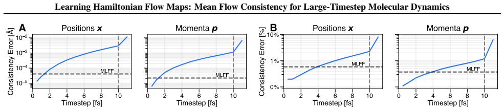
- [Appendix G.8, Figure 18] Figure 18 shows that the HFM's semigroup consistency error (u_Δt vs u_{Δt/2}∘u_{Δt/2}) grows beyond ~4 fs and is no longer comparable to Velocity Verlet at the production timesteps (9–12 fs). A true Hamiltonian flow map must satisfy the semigroup property exactly. The reported violation at the timesteps used in the main experiments indicates that the learned map deviates from the flow-map semigroup just where the method claims its advantage. Please report the semigroup error at the same Δt values as Table 15 and discuss why the violation does not degrade the equilibrium statistics, or restrict the flow-map claim to timesteps where the semigroup holds.
minor comments (5)
- [Appendix F.5] 'Totalling to 1 ms' should read 1 μs: 10 parallel simulations of 100 ns each sum to 1 μs, not 1 ms. Also check the unit for the source dataset description.
- [Appendix B.1, Eq. (23)] The mixture distribution q(τ) = 0.98B(1,2) + 0.02U(0,1) is written without defining the Beta distribution parameters. Specify the density or parameterization explicitly.
- [Appendix G.6, Eq. (88)] The normalization in Eq. (88) uses N as the number of integration substeps without defining it. Please define N and the indexing range.
- [Algorithm 3] Algorithm 3 includes a Thermostat step, but the NVE experiments presumably omit it. State this explicitly and clarify which filters are used in each ensemble.
- [§4.2, Eq. (10) and Algorithm 1] Eq. (10) writes a plain regression loss, while Algorithm 1 uses stop-gradient on the target. Align the notation so the reader knows the target is treated as a fixed regression target.
Circularity Check
No circularity: the mean-flow objective is a fixed-point consistency condition anchored by external force labels, with an in-paper sufficiency proof; self-citations are not load-bearing.
full rationale
I walked the derivation chain from Eq. (6) through Eq. (12) and Appendix C. Eq. (6) defines the true mean displacement field as the time-averaged Hamiltonian vector field; Eqs. (7)-(9) are a necessary differential consequence obtained by differentiation and Hamilton's equations. The training loss in Eq. (10) enforces this consistency condition, with the target computed from the network's own Jacobian-vector products. This is a self-consistency/fixed-point objective, not a circular prediction: the PDE has a unique solution given the Δt=0 boundary condition, and that boundary condition is anchored to external instantaneous force/velocity labels. Appendix C proves sufficiency by showing that any field satisfying the PDE and the Δt=0 boundary condition must equal the true time-averaged displacement; the integration-constant argument is mathematically standard and does not assume the conclusion. Eq. (12) is definitional (flow map = state + Δt·mean displacement), not a fitted result presented as independent. The self-citations in the paper (e.g., Frank et al. 2025 for the architecture, Plainer et al. 2025 as a baseline) are not load-bearing for the central claim; the consistency derivation and sufficiency proof are presented in the paper and build on external work (Geng et al., Boffi et al.). The acknowledged instability near Δt≈10 fs for alanine dipeptide (Section 5.2, Appendix G.11) is an empirical correctness/stability limitation concerning whether the loss is sufficiently minimized on the rollout distribution; it does not make the derivation equivalent to its inputs.
Assumptions & free parameters
free parameters (5)
- Δt_max (training horizon) =
10 fs (small molecules), 15 fs (alanine dipeptide), 2.5 (toys), 0.1 (N-body)
- q_Δt=0 = 0.75 (force-matching anchor probability) =
0.75
- Momenta sampling temperature distribution =
T ~ N(500 K, 150 K), clipped at 0
- Mixture timestep distribution q(τ) =
0.98·Beta(1,2) + 0.02·Uniform(0,1)
- Adaptive loss weights c=1e-3, p=0.5; λ_v=λ_f=1 =
c=1e-3, p=0.5, λ_v=λ_f=1
assumptions (6)
- domain assumption Hamilton's equations exactly describe the system; the Hamiltonian is time-independent (and separable for MD systems).
- domain assumption Force labels in the datasets are exact instantaneous forces from the true potential (ab initio or analytical).
- domain assumption A sufficiently expressive network can represent the mean displacement field, and minimizing the consistency loss with stop-gradient reaches the fixed point of Eq (8) on the training distribution.
- domain assumption Independent phase-space samples with momenta sampled from Maxwell-Boltzmann distributions are representative of the states visited during long rollouts.
- domain assumption The coupled energy/angular-momentum filter and the Langevin thermostat correct non-conservative errors without masking fundamental integration error.
- domain assumption Random rotation augmentation/filter approximately restores rotation equivariance without unduly stochasticizing NVE dynamics.
Cite this review
Pith. "Pith review of Learning Hamiltonian Flow Maps: Mean Flow Consistency for Large-Timestep Molecular Dynamics." pith.science (2026). https://pith.science/paper/247HM66Z
@misc{pith2026260122123,
  author       = {Pith},
  title        = {Pith review of: Learning Hamiltonian Flow Maps: Mean Flow Consistency for Large-Timestep Molecular Dynamics},
  year         = {2026},
  howpublished = {\url{https://pith.science/paper/247HM66Z}},
  note         = {Machine review of arXiv:2601.22123}
}
read the original abstract
Simulating the long-time evolution of Hamiltonian systems is limited by the small timesteps required for stable numerical integration. To overcome this constraint, we introduce a framework to learn Hamiltonian Flow Maps by predicting the mean phase-space evolution over a chosen time span, enabling stable large-timestep updates far beyond the stability limits of classical integrators. To this end, we impose a Mean Flow consistency condition for time-averaged Hamiltonian dynamics. Unlike prior approaches, this allows training on independent phase-space samples without access to future states, avoiding expensive trajectory generation. Validated across diverse Hamiltonian systems, our method in particular improves upon molecular dynamics simulations using machine-learned force fields (MLFF). Our models maintain comparable training and inference cost, but support significantly larger integration timesteps while trained directly on widely-available trajectory-free MLFF datasets.
Figures


Figures from the paper (19 more)




Forward citations
Cited by 1 Pith paper
-
Implicit Machine Learning Force Fields Accelerate Molecular Dynamics Simulations
Replacing explicit neural network stacks with self-consistent fixed-point iterations, and warm-starting the solver across timesteps, gives 2-5x cheaper molecular dynamics force evaluation at matched accuracy.
Reference graph
Works this paper leans on
-
[2007]
in Table 9 are comparable to those using the Langevin thermostat (Bussi & Parrinello, 2007) in Table 1. 32 Learning Hamiltonian Flow Maps: Mean Flow Consistency for Large-Timestep Molecular Dynamics Furthermore, during early experiments, we found that global momenta rescaling in global thermostats is generally less robust than local Langevin dynamics, as ...
2007
-
[2024]
We adopt the transformer architecture from Frank et al
(Apache-2.0). We adopt the transformer architecture from Frank et al. (2025) (MIT), which is implemented on top of e3x (Unke & Maennel, 2024) (Apache-2.0). For simulation utilities, we use ase (Larsen et al., 2017) (GNU LGPLv2.1). 21 Learning Hamiltonian Flow Maps: Mean Flow Consistency for Large-Timestep Molecular Dynamics C. Sufficiency of the Proposed ...
2025
-
[2265]
PMLR, 2015. 12 Learning Hamiltonian Flow Maps: Mean Flow Consistency for Large-Timestep Molecular Dynamics Song, Y . and Dhariwal, P. Improved techniques for train- ing consistency models. InThe Twelfth International Conference on Learning Representations, 2024. Song, Y ., Sohl-Dickstein, J., Kingma, D. P., Kumar, A., Er- mon, S., and Poole, B. Score-base...
arXiv 2015
Reviewed August 3, 2026 · model on record in the stance chip above.
Discussion (0). Continue with ORCID to comment.