REVIEW 4 major objections 6 minor 42 references
Numerical solutions of fixed points in two-dimensional Kuramoto-Sivashinsky equation expedited by reinforcement learning
T0 review · 4 major / 6 minor · reviewed 2026-08-10 · deepseek-v4-flash
Pith's one-line read A hybrid reinforcement-learning and Newton solver identifies 303 previously unreported fixed points of the two-dimensional Kuramoto-Sivashinsky equation, a canonical chaotic partial differential equation.
desk verdict A plausible method and a potentially valuable catalog, but the 303 fixed points claim is under-evidenced by the published tables. read the letter →
The pith
A machine-rendered reading of the paper's core claim, the machinery that carries it, and where it could break.
The reading
What carries the argument
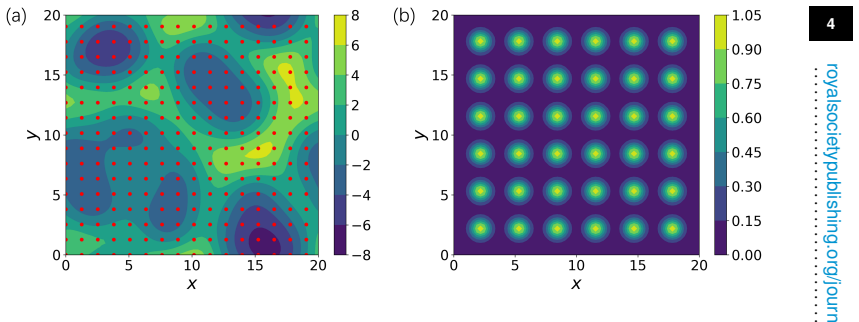
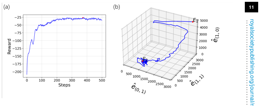
The load-bearing mechanism is the DRL-as-preconditioner loop. The reward function $r = -\|\mathrm{FFT}(u_{t+\Delta t}) - \mathrm{FFT}(u_t)\|_2$ acts as a spectral residual: it is zero exactly at a fixed point, where the unforced state reproduces itself after one time step, so states with high reward lie in the basin of convergence of JFNK. The actor-critic DDPG agent, with 256 sensor measurements and 36 Gaussian actuator amplitudes, searches this reward landscape over 500-step episodes, and the single best state per episode is handed to JFNK when its reward exceeds $\theta_{\mathrm{th}}=-45$. This matters because JFNK alone converges to a tolerance below $10^{-10}$ in successful cases but plateaus at residuals of order 0.1 to 1 in about two-thirds of 1500 random-start trials.
What would settle it
Recompute a sample of the reported equilibria, especially E27 and E28, at $128\times128$ Fourier resolution with time step 0.025, and compare the full Fourier spectra; if the high-wavenumber modes merge or the residual does not converge below $10^{-10}$, the stated catalog over-counts or mislabels distinct fixed points.
Extended reading notes
Core claim
On the paper's own terms, the central claim is a numerical discovery: the two-dimensional KSE on the square domain $[0,20]^2$ with periodic boundary conditions has at least 303 distinct steady solutions, all unstable, all previously absent from the literature. The route to this discovery is a two-stage method. First, a deep reinforcement learning agent, using 16x16 local sensors and 36 Gaussian actuators, is rewarded by the negative Fourier-space distance between the current state and its unforced evolution one time step later, namely $r = -\|\mathrm{FFT}(u_{t+\Delta t}) - \mathrm{FFT}(u_t)\|_2$; maximizing this reward drives the system toward states close to a fixed point. The best state found in an episode, when its reward exceeds the threshold $-45$, becomes the initial guess for JFNK, which then converges to the equilibrium proper. The paper also claims that the learned controller can navigate the system between known fixed points, stabilizing the trajectory near an unstable target.
Load-bearing premise
The numerical configuration of 64x64 Fourier modes with time step 0.05 on the $20\times20$ periodic domain faithfully captures every genuinely distinct fixed point of the continuous 2D KSE, including the high-wavenumber structure that tells E27 and E28 apart.
Editorial extensions
If this is right
- The 2D KSE in the chaotic regime at $2L=20$ possesses at least 303 invariant equilibria, giving a concrete target set for state-space analyses of spatiotemporal chaos.
- The DRL-enhanced initial guesses cut the average JFNK convergence iterations from 38.2 to 27.4 when both start from the same random seeds.
- The same reward function can be reused as a cheap fixed-point proximity oracle for other high-dimensional PDEs where Newton solvers fail without good initial guesses.
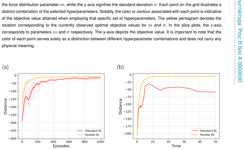
- The trained DRL controller can steer the 2D KSE from a random state to a chosen unstable fixed point and hold it there for at least 50 time units, within roughly 8 time units of actuation.
Reading between the lines
- If the 303 count survives higher-resolution checks, it is a lower bound, not a census; the dense clustering of low-mode signatures near the origin in Figure 9 hints that many more equilibria may await discovery by the same pipeline.
- The two entries E27 and E28 share identical values for the three tabulated low-order Fourier coefficients, yet no higher-order coefficients are given to separate them; a recomputation at $128\times128$ resolution would settle whether the catalog over-counts.
- Because the reward is computed in Fourier space with no forcing, the method is essentially a learned globalization strategy for Newton's method; the same idea could apply to finding other exact coherent structures, such as periodic orbits, by rewarding closeness to a recurrence rather than to a fixed point.
Editorial analysis
A structured set of objections, weighed in public.
Referee Report
Summary. This paper proposes a hybrid method in which deep reinforcement learning (DDPG) is used to generate improved initial guesses for a Jacobian-Free Newton-Krylov (JFNK) solver, applied to finding fixed points of the two-dimensional Kuramoto-Sivashinsky equation (2D KSE) on a 20-by-20 periodic domain with 64x64 Fourier collocation points. The authors report 303 distinct fixed points, claim that these are new and not previously reported, and also demonstrate DRL-based navigation between known fixed points. The numerical methods are standard: spectral spatial discretization, exponential time-differencing/RK4 time stepping, and a JFNK solver with stated tolerances. The core empirical claims are the 303-point catalogue in Tables 1 and 2 and the improved convergence of JFNK when initialized by DRL.
Significance. If the catalogue is correct, the paper provides a substantial numerical resource for studying equilibria of the 2D KSE in a chaotic regime, and it demonstrates a practical use of DRL as a preconditioning/initialization strategy for Newton-type solvers in high-dimensional dynamical systems. The public release of code is a positive feature, as is the use of a residual-based reward that avoids circular fitting of the fixed points. The main significance, however, depends entirely on the verifiability of the 303 distinct equilibria. As submitted, the tables do not supply enough information to verify either convergence or pairwise distinctness, so the central claim is not yet supported by the published record.
major comments (4)
- [Section 4(b), Tables 1 and 2] The central claim that Tables 1 and 2 list 303 distinct fixed points cannot be verified from the published data. For each point, Table 1 gives only the absolute values of three complex Fourier coefficients, and Table 2 gives seven additional magnitudes for E1-E17 only. Complex phases are never reported, so two physically different fields with identical magnitudes are indistinguishable in the tables, and two identical fields are also indistinguishable. The text even acknowledges this degeneracy ('in some cases the values of be(0,1), be(1,1), be(1,0) appear the same for distinct fixed points'), but the published record does not resolve the degeneracy for the full catalogue. To support the 303-count claim, the authors should deposit the full 64x64 Fourier fields (or all complex coefficients) for every listed point, together with a script that computes pairwise distances and verifies distinctness.
- [Table 1, rows E27 and E28] Rows E27 and E28 are numerically identical in all three reported magnitudes: (be(0,1), be(1,1), be(1,0)) = (0, 0, 6331.2). Table 2 provides no additional coefficients for these two rows. Since the paper itself notes that distinct fixed points can share these three magnitudes, the published information cannot distinguish between a typo, a duplicate entry, and two genuinely different solutions whose phase information was suppressed. Because the count of 303 rests on such distinctions, this specific case must be resolved explicitly in a revision.
- [Section 3(a) and Appendix A] No residual norms are reported for the individual fixed points. The paper states a JFNK relative error tolerance of 10^-12 and Appendix A says successful cases reduce the tolerance below 10^-10, but Tables 1 and 2 do not list the final relative residual for any of the 303 states. Without these data, the reader cannot confirm that each listed state is actually an equilibrium of the discretized 2D KSE to the claimed tolerance. The revision should either tabulate the final residuals or provide them in the public repository along with a verification script.
- [Section 3(a), validation of discretization] The grid-independence and time-step-independence checks are reported for a 25-time-unit integration, and the comparison with Kalogirou et al. [35] is made for a single steady state. This does not establish that all 303 converged states, which span a wide range of amplitudes and symmetry properties, are converged solutions of the continuous PDE. The authors should demonstrate for a representative subset of the catalogue, including high-amplitude and asymmetric states such as E135, that the fixed points are insensitive to increasing the resolution to 128x128 and decreasing the time step to 0.025, using the same JFNK convergence criterion.
minor comments (6)
- [Section 3(a), sensor locations] The sensor location set xs_i in {0,4,8,16...60} appears to be missing the value 12; it should probably read {0,4,8,12,...,60}. Please clarify.
- [Appendix A] The main text states a relative error tolerance of 10^-12, while Appendix A says successful cases reduce the tolerance to below 10^-10. These two statements should be reconciled or explained.
- [Section 3(a), Figure 2] Figure 2 compares the authors' result with a figure from Ref. [35], but the comparison is only visual. A quantitative error measure between the two steady states would strengthen the validation.
- [Table 1 caption] The caption says values are 'the absolute value of the first three complex-valued Fourier coefficients' and are not normalized, but it is not stated whether these values are raw magnitudes of the unnormalized FFT or scaled in some other way. Please define the normalization convention precisely in the caption or text.
- [References] There are several small reference formatting errors, for example 'Sivashinsk G' instead of Sivashinsky, and inconsistent capitalization in the Physical Review E entries. These should be cleaned up.
- [Section 4(b), Figures 8 and 9] Figure 8 states that E1 and E48 exhibit symmetry in x and y, while E81 and E135 are asymmetric. It would be helpful to quantify symmetry (for example, by reporting the residual under the relevant reflection operations) rather than relying on visual inspection.
Circularity Check
No significant circularity: the 2D KSE fixed points are solved from the PDE residual, and DRL only provides initial guesses; missing phase data is a verifiability issue, not circularity.
full rationale
The paper's central result—the 303 fixed points—is not obtained by fitting or by renaming inputs. The DRL reward (Eq. 3.3) is the negative L2 norm of the difference between the unforced state and its one-time-step evolution in Fourier space; this is exactly the residual whose zero defines a fixed point of the numerical flow. The JFNK solver (adapted from the independent code of Willis, Ref. [36]) then drives the same residual to a relative tolerance of 10^-12 (Section 3(a)). Thus the listed states are solutions of the discretized KSE equations, not fitted or definitionally forced outputs. DRL hyperparameters (m, sigma, alpha_min) are tuned and affect which initial guesses are generated, but they do not enter the fixed-point equations or the reported solutions. The comparison to Kalogirou et al. [35] and the grid/time-step independence checks provide external anchors. References [26] and [27] involve the corresponding author's group, but they are cited only as examples of DRL flow control and do not justify the fixed-point results. The only notable defect is evidential rather than circular: Section 4(b) and Table 1 report only the absolute values of three Fourier coefficients for most states, and rows E27 and E28 are numerically identical (0, 0, 6331.2), with no Table 2 entries provided to distinguish them. The authors note that 'in some cases the values of be(0,1), be(1,1), be(1,0) appear the same for distinct fixed points. Under these circumstances, more Fourier coefficients will be provided to differentiate them (see table 2),' but for E27/E28 this is not done. This means the '303 distinct' claim cannot be independently verified from the published tables; it is an omitted-data/correctness concern, not a reduction of the derivation to its own inputs.
Assumptions & free parameters
free parameters (4)
- Reward threshold theta_th =
-45
- Minimum exploration noise alpha_min (navigation) =
1.2
- Actuator count m =
6
- Actuator width sigma =
2.4
assumptions (3)
- domain assumption The 2D KSE on [0,20]^2 with periodic boundary conditions is an adequate model of the chaotic dynamics of interest.
- domain assumption The spectral discretization with N=64x64 and time step 0.05 accurately resolves all fixed points of the continuous PDE.
- standard math A JFNK residual below 10^-10 implies a genuine fixed point of the discretized system.
Cite this review
Pith. "Pith review of Numerical solutions of fixed points in two-dimensional Kuramoto-Sivashinsky equation expedited by reinforcement learning." pith.science (2026). https://pith.science/paper/YT65BZBS
@misc{pith2026250100046,
  author       = {Pith},
  title        = {Pith review of: Numerical solutions of fixed points in two-dimensional Kuramoto-Sivashinsky equation expedited by reinforcement learning},
  year         = {2026},
  howpublished = {\url{https://pith.science/paper/YT65BZBS}},
  note         = {Machine review of arXiv:2501.00046}
}
read the original abstract
This paper presents a combined approach to enhancing the effectiveness of Jacobian-Free Newton-Krylov (JFNK) method by deep reinforcement learning (DRL) in identifying fixed points within the 2D Kuramoto-Sivashinsky Equation (KSE). JFNK approach entails a good initial guess for improved convergence when searching for fixed points. With a properly defined reward function, we utilise DRL as a preliminary step to enhance the initial guess in the converging process. We report new results of fixed points in the 2D KSE which have not been reported in the literature. Additionally, we explored control optimization for the 2D KSE to navigate the system trajectories between known fixed points, based on parallel reinforcement learning techniques. This combined method underscores the improved JFNK approach to finding new fixed-point solutions within the context of 2D KSE, which may be instructive for other high-dimensional dynamical systems.
Figures


Figures from the paper (11 more)




Reference graph
Works this paper leans on
-
[35]
2015 An in-depth numerical study of the two- dimensional Kuramoto–Sivashinsky equation
Kalogirou A, Keaveny EE, Papageorgiou DT. 2015 An in-depth numerical study of the two- dimensional Kuramoto–Sivashinsky equation. Proceedings of the Royal Society A: Mathematical, Physical and Engineering Sciences 471, 20140932
work page 2015
-
[1]
1986 The Kuramoto-Sivashinsky equation: a bridge between PDE’s and dynamical systems
Hyman JM, Nicolaenko B. 1986 The Kuramoto-Sivashinsky equation: a bridge between PDE’s and dynamical systems. Physica D: Nonlinear Phenomena 18, 113–126
work page 1986
-
[2]
2010 On the state space geometry of the Kuramoto– Sivashinsky flow in a periodic domain
Cvitanovi´ c P , Davidchack RL, Siminos E. 2010 On the state space geometry of the Kuramoto– Sivashinsky flow in a periodic domain. SIAM Journal on Applied Dynamical Systems 9, 1–33
work page 2010
-
[3]
Kuramoto Y, Tsuzuki T. 1975 On the formation of dissipative structures in reaction-diffusion systems: Reductive perturbation approach. Progress of Theoretical Physics 54, 687–699
work page 1975
-
[4]
1988 Nonlinear analysis of hydrodynamic instability in laminar flames—I
Sivashinsk G. 1988 Nonlinear analysis of hydrodynamic instability in laminar flames—I. Derivation of basic equations. In Dynamics of Curved Fronts , pp. 459–488. Elsevier
work page 1988
-
[5]
2014 Nonlinear dynamics and chaos: With applications to physics, biology, chemistry, and engineering
Strogatz SH. 2014 Nonlinear dynamics and chaos: With applications to physics, biology, chemistry, and engineering. Westview Press 2nd edition
work page 2014
-
[6]
1982 The strange attractor theory of turbulence.Annual Review of Fluid Mechanics 14, 347–364
Lanford III O. 1982 The strange attractor theory of turbulence.Annual Review of Fluid Mechanics 14, 347–364
work page 1982
-
[7]
2005 Recent progress in understanding the transition to turbulence in a pipe
Kerswell RR. 2005 Recent progress in understanding the transition to turbulence in a pipe. Nonlinearity 18, R17
work page 2005
Show all 42 references
-
[8]
2011 The Significance of Simple Invariant Solutions in Turbulent Flows
Kawahara G, Uhlmann M, van Veen L. 2011 The Significance of Simple Invariant Solutions in Turbulent Flows. Annual Review of Fluid Mechanics 44, 203–225
2011
-
[9]
2021 Exact Coherent States and the Nonlinear Dynamics of Wall- Bounded Turbulent Flows
Graham MD, Floryan D. 2021 Exact Coherent States and the Nonlinear Dynamics of Wall- Bounded Turbulent Flows. Annual Review of Fluid Mechanics 53, 227–253
2021
-
[10]
1986 The well-posedness of the Kuramoto–Sivashinsky equation
Tadmor E. 1986 The well-posedness of the Kuramoto–Sivashinsky equation. SIAM Journal on Mathematical analysis 17, 884–893
1986
-
[11]
1991 Predicting chaos for infinite dimensional dynamical systems: the Kuramoto-Sivashinsky equation, a case study..Proceedings of the National Academy of Sciences 88, 11129–11132
Smyrlis YS, Papageorgiou DT. 1991 Predicting chaos for infinite dimensional dynamical systems: the Kuramoto-Sivashinsky equation, a case study..Proceedings of the National Academy of Sciences 88, 11129–11132
1991
-
[12]
1990 Back in the saddle again: a computer assisted study of the Kuramoto–Sivashinsky equation
Kevrekidis IG, Nicolaenko B, Scovel JC. 1990 Back in the saddle again: a computer assisted study of the Kuramoto–Sivashinsky equation. SIAM Journal on Applied Mathematics 50, 760– 790
1990
-
[13]
2019 Linearly recurrent autoencoder networks for learning dynamics
Otto SE, Rowley CW. 2019 Linearly recurrent autoencoder networks for learning dynamics. SIAM Journal on Applied Dynamical Systems 18, 558–593
2019
-
[14]
1988 The steady states of the Kuramoto-Sivashinsky equation
Greene J, Kim JS. 1988 The steady states of the Kuramoto-Sivashinsky equation. Physica D: Nonlinear Phenomena 33, 99–120
1988
-
[15]
2008 Unstable recurrent patterns in Kuramoto-Sivashinsky dynamics
Lan Y, Cvitanovi´ c P . 2008 Unstable recurrent patterns in Kuramoto-Sivashinsky dynamics. Physical review E 78, 026208
2008
-
[16]
2004 Jacobian-free Newton–Krylov methods: a survey of approaches and applications
Knoll DA, Keyes DE. 2004 Jacobian-free Newton–Krylov methods: a survey of approaches and applications. Journal of Computational Physics 193, 357–397
2004
-
[17]
2017 Asymmetric actor critic for image-based robot learning
Pinto L, Andrychowicz M, Welinder P , Zaremba W, Abbeel P . 2017 Asymmetric actor critic for image-based robot learning. arXiv preprint arXiv:1710.06542
2017 arXiv
-
[18]
2016 An actor-critic algorithm for sequence prediction
Bahdanau D, Brakel P , Xu K, Goyal A, Lowe R, Pineau J, Courville A, Bengio Y. 2016 An actor-critic algorithm for sequence prediction. arXiv preprint arXiv:1607.07086
2016 arXiv
-
[19]
2013 Playing atari with deep reinforcement learning
Mnih V , Kavukcuoglu K, Silver D, Graves A, Antonoglou I, Wierstra D, Riedmiller M. 2013 Playing atari with deep reinforcement learning. arXiv preprint arXiv:1312.5602
2013 arXiv
-
[20]
2017 Mastering the game of go without human knowledge
Silver D, Schrittwieser J, Simonyan K, Antonoglou I, Huang A, Guez A, Hubert T, Baker L, Lai M, Bolton A et al.. 2017 Mastering the game of go without human knowledge. nature 550, 354–359
2017
-
[21]
2019 Learning to drive in a day
Kendall A, Hawke J, Janz D, Mazur P , Reda D, Allen JM, Lam VD, Bewley A, Shah A. 2019 Learning to drive in a day. In 2019 International Conference on Robotics and Automation (ICRA) pp. 8248–8254. IEEE
2019
-
[22]
2020 Machine Learning for Fluid Mechanics.Annual Review of Fluid Mechanics 52, 477–508
Brunton SL, Noack BR, Koumoutsakos P . 2020 Machine Learning for Fluid Mechanics.Annual Review of Fluid Mechanics 52, 477–508
2020
-
[23]
2020 Deep reinforcement learning in fluid mechanics: A promising method for both active flow control and shape optimization
Rabault J, Ren F, Zhang W, Tang H, Xu H. 2020 Deep reinforcement learning in fluid mechanics: A promising method for both active flow control and shape optimization. Journal of Hydrodynamics 32, 234–246. 22royalsocietypublishing.org/journal/rspa Proc R Soc A 0000000
2020
-
[24]
2019 Artificial neural networks trained through deep reinforcement learning discover control strategies for active flow control.Journal of fluid mechanics 865, 281–302
Rabault J, Kuchta M, Jensen A, Réglade U, Cerardi N. 2019 Artificial neural networks trained through deep reinforcement learning discover control strategies for active flow control.Journal of fluid mechanics 865, 281–302
2019
-
[25]
2021 Robust flow control and optimal sensor placement using deep reinforcement learning
Paris R, Beneddine S, Dandois J. 2021 Robust flow control and optimal sensor placement using deep reinforcement learning. Journal of Fluid Mechanics 913, A25
2021
-
[26]
2022 Reinforcement-learning-based control of confined cylinder wakes with stability analyses
Li J, Zhang M. 2022 Reinforcement-learning-based control of confined cylinder wakes with stability analyses. Journal of Fluid Mechanics 932, A44
2022
-
[27]
2023 Reinforcement-learning-based control of convectively unstable flows
Xu D, Zhang M. 2023 Reinforcement-learning-based control of convectively unstable flows. Journal of Fluid Mechanics 954, A37
2023
-
[28]
2023 Reinforcement learning of control strategies for reducing skin friction drag in a fully developed turbulent channel flow
Sonoda T, Liu Z, Itoh T, Hasegawa Y. 2023 Reinforcement learning of control strategies for reducing skin friction drag in a fully developed turbulent channel flow. Journal of Fluid Mechanics 960, A30
2023
-
[29]
2020 Controlling Rayleigh–Bénard convection via reinforcement learning
Beintema G, Corbetta A, Biferale L, Toschi F. 2020 Controlling Rayleigh–Bénard convection via reinforcement learning. Journal of Turbulence 21, 585–605
2020
-
[30]
2018 On-line building energy optimization using deep reinforcement learning.IEEE transactions on smart grid 10, 3698–3708
Mocanu E, Mocanu DC, Nguyen PH, Liotta A, Webber ME, Gibescu M, Slootweg JG. 2018 On-line building energy optimization using deep reinforcement learning.IEEE transactions on smart grid 10, 3698–3708
2018
-
[31]
2020 Reinforcement learning for bluff body active flow control in experiments and simulations
Fan D, Yang L, Wang Z, Triantafyllou MS, Karniadakis GE. 2020 Reinforcement learning for bluff body active flow control in experiments and simulations. Proceedings of the National Academy of Sciences 117, 26091–26098
2020
-
[32]
2021 Symmetry reduction for deep reinforcement learning active control of chaotic spatiotemporal dynamics
Zeng K, Graham MD. 2021 Symmetry reduction for deep reinforcement learning active control of chaotic spatiotemporal dynamics. Physical Review E 104, 014210
2021
-
[33]
2019 Control of chaotic systems by deep reinforcement learning
Bucci MA, Semeraro O, Allauzen A, Wisniewski G, Cordier L, Mathelin L. 2019 Control of chaotic systems by deep reinforcement learning. Proceedings of the Royal Society A 475, 20190351
2019
-
[34]
2005 Fourth-order time-stepping for stiff PDEs
Kassam AK, Trefethen LN. 2005 Fourth-order time-stepping for stiff PDEs. SIAM Journal on Scientific Computing 26, 1214–1233
2005
-
[36]
2019 Equilibria, periodic orbits and computing them
Willis AP . 2019 Equilibria, periodic orbits and computing them. arXiv preprint arXiv:1908.06730
2019 arXiv
-
[37]
2014 Deterministic policy gradient algorithms
Silver D, Lever G, Heess N, Degris T, Wierstra D, Riedmiller M. 2014 Deterministic policy gradient algorithms. In International conference on machine learning pp. 387–395. Pmlr
2014
-
[38]
2015 Continuous control with deep reinforcement learning
Lillicrap TP , Hunt JJ, Pritzel A, Heess N, Erez T, Tassa Y, Silver D, Wierstra D. 2015 Continuous control with deep reinforcement learning. arXiv preprint arXiv:1509.02971
2015 arXiv
-
[39]
2017 Surfing the edge: using feedback control to find nonlinear solutions
Willis AP , Duguet Y, Omel’chenko O, Wolfrum M. 2017 Surfing the edge: using feedback control to find nonlinear solutions. Journal of Fluid Mechanics 831, 579–591
2017
-
[40]
2018 A tutorial on Bayesian optimization
Frazier PI. 2018 A tutorial on Bayesian optimization. arXiv preprint arXiv:1807.02811
2018 arXiv
-
[41]
2012 Practical bayesian optimization of machine learning algorithms
Snoek J, Larochelle H, Adams RP . 2012 Practical bayesian optimization of machine learning algorithms. Advances in neural information processing systems 25
2012
-
[42]
2015 Scalable bayesian optimization using deep neural networks
Snoek J, Rippel O, Swersky K, Kiros R, Satish N, Sundaram N, Patwary M, Prabhat M, Adams R. 2015 Scalable bayesian optimization using deep neural networks. In International conference on machine learning pp. 2171–2180. PMLR
2015
Reviewed August 10, 2026 · model on record in the stance chip above.
Discussion (0). Continue with ORCID to comment.