REVIEW 3 major objections 7 minor 20 references
An Analysis of Model Robustness across Concurrent Distribution Shifts
T0 review · 3 major / 7 minor · reviewed 2026-08-10 · deepseek-v4-flash
Pith's one-line read This paper claims that when distribution shifts occur together, models degrade more than under any single shift, except that spurious correlation dominates so completely that adding extra shifts barely changes accuracy.
desk verdict Controlled ConDS benchmark is solid and useful; the real-world ConDS claim is asserted, not verified, and needs to be reined in before this can be accepted. read the letter →
The pith
A machine-rendered reading of the paper's core claim, the machinery that carries it, and where it could break.
The reading
What carries the argument
The central machinery is the ConDS protocol: a dataset is treated as instances generated from a finite set of attributes, with one attribute designated as label; shifts are created by manipulating how attribute values are distributed between source and target. UniDS consists of spurious correlation (SC), low data drift (LDD), and unseen data shift (UDS); ConDS is the set of all combinations of two or three of these, each applied to a different attribute. This lets the paper create 168 source-target pairs from five controlled and three real-world datasets and evaluate 26 algorithms under identical, standardized conditions.
What would settle it
On a controlled multi-attribute dataset, construct SC using attribute A and add a strong LDD using attribute B that is causally independent of A; if most algorithms show a large accuracy drop from SC alone to SC+LDD (comparable to the LDD-only drop), then the claim that SC masks additional shifts is false.
Extended reading notes
Core claim
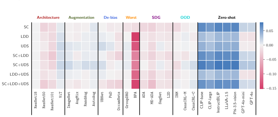
On the paper's own terms, the central discovery is that concurrent distribution shifts (ConDS) are typically more challenging than single distribution shifts, but spurious correlation (SC) dominates the difficulty: average accuracy under SC alone is close to that under SC+LDD and SC+UDS, and even under SC+LDD+UDS, while LDD+UDS without SC does show additional degradation. The paper also discovers that generalization benefits transfer across shift types—a method designed for one shift tends to help others—and that heuristic augmentations such as AugMix, RandAug, and AutoAug achieve the best overall performance on both synthetic and real-world benchmarks. Finally, zero-shot foundation models (CLIP, LLaVA, GPT-4o) perform well on controlled datasets but drop sharply on real-world datasets, with average accuracy falling from about 82% to 32%.
Load-bearing premise
The claim that real-world datasets exhibit the same concurrent shifts as the controlled ones rests on the assumption that iWildCam, fMoW, and Camelyon17 actually contain the specific LDD and UDS components the framework targets, which the paper does not explicitly verify.
Editorial extensions
If this is right
- Deployment under compound shifts is riskier than single-shift benchmarks suggest; models should be stress-tested with several concurrent shifts before release.
- Because spurious correlation dominates, accuracy improvements on non-spurious shifts may be invisible in overall averages; measuring performance on SC-heavy test sets is necessary to expose real robustness.
- The transfer of generalization gains across shift types means a single robust method can serve across multiple shift categories, reducing the need for shift-specific tuning.
- Heuristic augmentations and pre-training are the most cost-effective robustness levers among the 26 methods tested, outperforming more complex debiasing and domain-generalization losses.
- Foundation models' strong controlled-dataset performance does not carry over to niche or specialized real-world data; their use there needs fine-tuning or careful prompt design.
Reading between the lines
- Not tested in the paper: measuring worst-case shift accuracy instead of mean accuracy would likely reveal that SC-free shifts are where methods actually separate, since SC dominates the average.
- The ConDS protocol could be applied to continuous or learned attribute representations—e.g., clusters from self-supervised features—to test whether the SC > UDS > LDD difficulty ordering survives beyond the specific discrete attributes chosen.
- The paper's cross-shift transfer finding hints that robustness methods may share a common effect of increasing effective training diversity; isolating that effect could yield simpler methods than the bespoke losses evaluated.
Editorial analysis
A structured set of objections, weighed in public.
Referee Report
Summary. This paper introduces ConDS, an empirical benchmark for concurrent distribution shifts. The authors define UniDS as spurious correlation (SC), low data drift (LDD), and unseen data shift (UDS), and define ConDS as combinations of two or more UniDS applied to different attributes of a multi-attribute dataset. They construct 165 controlled source-target pairs from dSprites, Shapes3D, SmallNorb, CelebA, and DeepFashion, plus three real-world WILDS datasets (iWildCam, fMoW, Camelyon17), and evaluate a broad set of algorithms ranging from standard architectures and heuristic augmentations to zero-shot vision-language models. The main findings are that concurrent shifts are on average harder than single shifts, spurious correlations dominate so that adding LDD or UDS to SC yields little additional degradation, robustness generalizes across shift types, heuristic augmentations and pre-training are the most effective strategies, and zero-shot foundation models deteriorate on real-world datasets.
Significance. If the controlled results hold, the paper provides a useful and much-needed benchmark for compound distribution shifts, an area that is less studied than single shifts. Its strengths include the large standardized evaluation over many algorithms and datasets, the explicit controlled construction from attribute-annotated data, detailed per-dataset and per-algorithm results in the appendix, and public code. The paper is also honest about several limitations, such as the uniform test distribution and the limited number of attributes. The controlled-dataset findings are measured rather than derived, so there is no circularity concern. The main risk is that the real-world conclusions currently rest on an unverified assumption that WILDS datasets exhibit decomposable concurrent shifts, and the headline difficulty comparisons are based on only two controlled datasets.
major comments (3)
- [Section 5.1, Section 3.3, Table 3 caption] The treatment of iWildCam, fMoW, and Camelyon17 as 'real-world datasets with ConDS' is asserted rather than verified. Section 5.1 states that iWildCam 'exhibits LDD over the animal distributions, and UDS occurs across camera trap locations' and that fMoW 'exhibits UDS and LDD across time and regions in satellite images,' but no measurement separates these components or establishes that they co-occur independently. The manuscript itself concedes in Section 5.2 that 'Real-world datasets do not exhibit a clear distribution shift like controlled datasets, but they inherently contain various naturally occurring distribution shifts that may go unnoticed.' If, for example, the label imbalance in iWildCam is induced by the same camera-location mechanism that causes the image-style shift, then this is one entangled shift rather than two concurrent UniDS components, and the real-world extension of Takeaway 1 (and the real-world parts of Takeaways 4 and 6) is unsupported. Please either verify the decomposition with domain metadata (for instance, evaluating on subsets that vary one factor at a time) or explicitly label these datasets as 'assumed concurrent' and qualify the real-world claims accordingly.
- [Section 5.2, Figure 4] Takeaways 1 and 2 are stated as general claims, but the standardized difficulty comparison in Figure 4 'primarily relies on the Dsprites and CelebA' (Section 5.2). These are only two of the five controlled datasets. The aggregate plot in Figure 3 includes all five, but it mixes unequal dataset sizes and does not isolate the number-of-shifts effect. Please either report the standardized comparison for all five controlled datasets or explicitly restrict Takeaways 1 and 2 to dSprites and CelebA, and provide paired error bars or confidence intervals so that the 'ConDS is more challenging' claim is supported quantitatively.
- [Section 5.3, Takeaway 3] The claim that 'if a method improves generalization for one DS, it tends to be effective for others' is a central abstract claim, but the supporting evidence is only visual inspection of Figure 3. Given the large result matrix, the paper should quantify this consistency, for example by reporting rank correlations of algorithm accuracies across DS conditions and across datasets, with confidence intervals. Without such a measure, the 'tends to' claim is not falsifiable.
minor comments (7)
- [Section 5.2] The first paragraph says the paper evaluates '168 (source, target) pairs spanning six datasets,' but the paper uses eight datasets (five controlled plus three real-world), and the text later says there are 165 controlled pairs. Please reconcile the counts and clarify that 165 refers to the controlled datasets and 168 includes the three real-world pairs.
- [Table 1 and Section 4] Table 1 lists 28 model variants if CLIP-base and CLIP-large are counted separately (and 27 if CLIP is counted as one entry), while the text and abstract say 26 algorithms. Please make the algorithm count consistent between the text and the table.
- [Introduction] The citation 'CelebA (Karras et al., 2017)' is incorrect; the standard reference for CelebA is Liu et al., 2015, 'Deep Learning Face Attributes in the Wild'.
- [Section B.8] The phrase 'for the rebuttal' appears to be a leftover from the review process and should be removed or rephrased.
- [Section 5.2] The prompt citation '(Matsuura et al.)' lacks a year and a full reference entry; please add it to the bibliography.
- [Figure 3 caption] The sentence about zero-shot models having 'the same absolute performance for each row' is confusing, since the figure shows relative performance; please rewrite it.
- [Section B.11 and Takeaway 2] There are small typos: 'Computaional Cost' should be 'Computational Cost,' and 'Furthemore' should be 'Furthermore.'
Circularity Check
No circularity: the ConDS difficulty claims are measured accuracies, not consequences of the ConDS definition.
full rationale
This is an empirical benchmarking paper. Its central claims (ConDS typically harder than UniDS; SC dominates; augmentations are best overall) are measurements over 168 source-target pairs on external datasets, not consequences of the formal definition. Equation (3) defines ConDS as subsets of UniDS of size at least 2, but the finding that adding more shifts usually lowers accuracy, and that SC saturates the drop, is an observed empirical ordering; nothing is fitted and then renamed a prediction. The UniDS definitions are imported from Wiles et al. (2022), an external benchmark, and used only to name shift types; the actual construction is detailed in Section A.2. The paper does contain an admitted limitation: Section 5.2 says 'Real-world datasets do not exhibit a clear distribution shift like controlled datasets, but they inherently contain various naturally occurring distribution shifts that may go unnoticed,' and Section 5.1 asserts without separate measurement that iWildCam and fMoW exhibit LDD and UDS components. That is an external-validity or correctness risk for the real-world generalization of Takeaway 4, not circularity: the controlled experiments stand independently, and the real-world claim is an unverified assumption rather than a derivation that reduces to its own inputs. No self-citation is load-bearing: Jeon et al. (2022a) is cited only for the 1% counterexample setup convention in SC construction, and Koh et al. (2021) is an external prior benchmark. Verdict: no significant circularity, score 0.
Assumptions & free parameters
free parameters (1)
- Per-algorithm hyperparameters (learning rate, augmentation magnitudes, etc.) =
Selected by grid search per dataset and shift; detailed in Table 9
assumptions (3)
- domain assumption Test distribution pT is uniform over all attribute values
- domain assumption Real-world datasets iWildCam, fMoW, and Camelyon17 contain the specific concurrent DSs under study
- ad hoc to paper Spurious correlation source data include 1% counterexamples
Cite this review
Pith. "Pith review of An Analysis of Model Robustness across Concurrent Distribution Shifts." pith.science (2026). https://pith.science/paper/YP7JJRAL
@misc{pith2026250104288,
  author       = {Pith},
  title        = {Pith review of: An Analysis of Model Robustness across Concurrent Distribution Shifts},
  year         = {2026},
  howpublished = {\url{https://pith.science/paper/YP7JJRAL}},
  note         = {Machine review of arXiv:2501.04288}
}
read the original abstract
Machine learning models, meticulously optimized for source data, often fail to predict target data when faced with distribution shifts (DSs). Previous benchmarking studies, though extensive, have mainly focused on simple DSs. Recognizing that DSs often occur in more complex forms in real-world scenarios, we broadened our study to include multiple concurrent shifts, such as unseen domain shifts combined with spurious correlations. We evaluated 26 algorithms that range from simple heuristic augmentations to zero-shot inference using foundation models, across 168 source-target pairs from eight datasets. Our analysis of over 100K models reveals that (i) concurrent DSs typically worsen performance compared to a single shift, with certain exceptions, (ii) if a model improves generalization for one distribution shift, it tends to be effective for others, and (iii) heuristic data augmentations achieve the best overall performance on both synthetic and real-world datasets.
Figures


Figures from the paper (37 more)




Reference graph
Works this paper leans on
-
[1]
Marah Abdin, Sam Ade Jacobs, Ammar Ahmad Awan, Jyoti Aneja, Ahmed Awadallah, Hany Awadalla, Nguyen Bach, Amit Bahree, Arash Bakhtiari, Harkirat Behl, et al. Phi-3 technical report: A highly capable language model locally on your phone.arXiv preprint arXiv:2404.14219,
-
[3]
iWildCam fMoW Camelyon17 Scratch Pre-training Scratch Pre-training Scratch Pre-training Architecture ResNet18 51.77(±0.47) 59.50(±0.43) 27.13(±0.44) 41.08(±0.44) 82.83(±0.25) 84.35(±0.10) ResNet50 53.35(±0.34) 66.75(±0.39) 28.55(±0.44) 49.75(±0.32) 75.85(±0.36) 86.78(±0.38) ResNet101 43.41(±0.07) 69.71(±0.20) 22.35(±0.30) 48.63(±0.17) 75.26(±0.37) 84.21(±...
work page 2022
-
[7]
In search of lost domain generalization
Ishaan Gulrajani and David Lopez-Paz. In search of lost domain generalization. arXiv preprint arXiv:2007.01434,
arXiv 2007
-
[8]
Benchmarking neural network robustness to common corruptions and perturbations
Dan Hendrycks and Thomas Dietterich. Benchmarking neural network robustness to common corruptions and perturbations. arXiv preprint arXiv:1903.12261,
arXiv 1903
-
[9]
Augmix: A simple data processing method to improve robustness and uncertainty
Dan Hendrycks, Norman Mu, Ekin D Cubuk, Barret Zoph, Justin Gilmer, and Balaji Lakshminarayanan. Augmix: A simple data processing method to improve robustness and uncertainty. arXiv preprint arXiv:1912.02781,
arXiv 1912
-
[11]
Improved baselines with visual instruction tuning
Haotian Liu, Chunyuan Li, Yuheng Li, and Yong Jae Lee. Improved baselines with visual instruction tuning. arXiv preprint arXiv:2310.03744,
-
[12]
Visual-llm zero-shot classification
Misaki Matsuura, Young Kyun Jung, and Ser Nam Lim. Visual-llm zero-shot classification. Leland McInnes, John Healy, and James Melville. Umap: Uniform manifold approximation and projection for dimension reduction.arXiv preprint arXiv:1802.03426,
-
[13]
Accessed: 2024-05-26. Maxime Oquab, Timothée Darcet, Théo Moutakanni, Huy Vo, Marc Szafraniec, Vasil Khalidov, Pierre Fernandez, Daniel Haziza, Francisco Massa, Alaaeldin El-Nouby, Mahmoud Assran, Nicolas Ballas, Woj- ciech Galuba, Russell Howes, Po-Yao Huang, Shang-Wen Li, Ishan Misra, Michael Rabbat, Vasu Sharma, Gabriel Synnaeve, Hu Xu, Hervé Jegou, Ju...
work page 2024
Show all 20 references
-
[14]
Distributionally robust neural networks for group shifts: On the importance of regularization for worst-case generalization.arXiv preprint arXiv:1911.08731,
Shiori Sagawa, Pang Wei Koh, Tatsunori B Hashimoto, and Percy Liang. Distributionally robust neural networks for group shifts: On the importance of regularization for worst-case generalization.arXiv preprint arXiv:1911.08731,
1911 arXiv
-
[15]
A systematic survey of prompt engineering in large language models: Techniques and applications.arXiv preprint arXiv:2402.07927,
14 Pranab Sahoo, Ayush Kumar Singh, Sriparna Saha, Vinija Jain, Samrat Mondal, and Aman Chadha. A systematic survey of prompt engineering in large language models: Techniques and applications.arXiv preprint arXiv:2402.07927,
-
[16]
A fine-grained analysis on distribution shift.arXiv preprint arXiv:2110.11328,
Olivia Wiles, Sven Gowal, Florian Stimberg, Sylvestre Alvise-Rebuffi, Ira Ktena, Krishnamurthy Dvijotham, and Taylan Cemgil. A fine-grained analysis on distribution shift.arXiv preprint arXiv:2110.11328,
-
[17]
Shen Yan, Huan Song, Nanxiang Li, Lincan Zou, and Liu Ren
URL https://openreview.net/forum?id=Dl4LetuLdyK. Shen Yan, Huan Song, Nanxiang Li, Lincan Zou, and Liu Ren. Improve unsupervised domain adaptation with mixup training.arXiv preprint arXiv:2001.00677,
2001 arXiv
-
[19]
Table 14:Fine-tuned open source foundation model.w and w/o denote with and without fine-tuning, respectively. iWildCam Camelyon17 FMoW w/o w w/o w w/o w LLaVA-1.54.64 91.1251.0995.3216.3272.67 Phi-3.5-Vision9.91 91.1966.7193.3510.8877.02 InstructBLIP1.86 12.1368.0399.8718.1741...
1966
-
[21]
However, such datasets are limited as annotations are expensive
31 B.8 Generation of Attributes with Augmentations Our framework requires datasets with rich attribute annotations to createConDS. However, such datasets are limited as annotations are expensive. We did consider using augmentations to create additional attribu- tions, but augm...
2018
-
[2016]
Imagenet-trained cnns are biased towards texture; increasing shape bias improves accuracy and robustness
12 Robert Geirhos, Patricia Rubisch, Claudio Michaelis, Matthias Bethge, Felix A Wichmann, and Wieland Brendel. Imagenet-trained cnns are biased towards texture; increasing shape bias improves accuracy and robustness. arXiv preprint arXiv:1811.12231,
-
[2018]
Invariant risk minimization.arXiv preprint arXiv:1907.02893,
Martin Arjovsky, Léon Bottou, Ishaan Gulrajani, and David Lopez-Paz. Invariant risk minimization.arXiv preprint arXiv:1907.02893,
1907 arXiv
-
[2019]
Pali: A jointly-scaled multilingual language-image model
Xi Chen, Xiao Wang, Soravit Changpinyo, AJ Piergiovanni, Piotr Padlewski, Daniel Salz, Sebastian Good- man, Adam Grycner, Basil Mustafa, Lucas Beyer, et al. Pali: A jointly-scaled multilingual language-image model. arXiv preprint arXiv:2209.06794,
-
[2022]
Invariant causal mechanisms through distribution matching.arXiv preprint arXiv:2206.11646,
Mathieu Chevalley, Charlotte Bunne, Andreas Krause, and Stefan Bauer. Invariant causal mechanisms through distribution matching.arXiv preprint arXiv:2206.11646,
-
[2023]
Progressive growing of gans for improved quality, stability, and variation.arXiv preprint arXiv:1710.10196,
Tero Karras, Timo Aila, Samuli Laine, and Jaakko Lehtinen. Progressive growing of gans for improved quality, stability, and variation.arXiv preprint arXiv:1710.10196,
-
[2024]
An image is worth 16x16 words: Transformers for image recognition at scale.arXiv preprint arXiv:2010.11929,
Alexey Dosovitskiy, Lucas Beyer, Alexander Kolesnikov, Dirk Weissenborn, Xiaohua Zhai, Thomas Un- terthiner, Mostafa Dehghani, Matthias Minderer, Georg Heigold, Sylvain Gelly, et al. An image is worth 16x16 words: Transformers for image recognition at scale.arXiv preprint arXi...
2010 arXiv
Reviewed August 10, 2026 · model on record in the stance chip above.
Discussion (0). Continue with ORCID to comment.