REVIEW 1 major objections 8 minor 43 references
Load Forecasting for Households and Energy Communities: Are Deep Learning Models Worth the Effort?
T0 review · 1 major / 8 minor · reviewed 2026-08-10 · deepseek-v4-flash
Pith's one-line read For energy-community load forecasting, deep learning is not always worth the effort: with fewer than six months of training data, persistence forecasting is more accurate, and a simple KNN model nearly matches the best deep learning…
desk verdict A useful, reproducible empirical benchmark with a practical data-threshold finding, but the headline six-month persistence advantage is tested on one season only and the text overstates the nine-month improvement. read the letter →
The pith
A machine-rendered reading of the paper's core claim, the machinery that carries it, and where it could break.
The reading
What carries the argument
The argument is carried by a controlled sensitivity grid: each configuration is evaluated on 20 randomly drawn virtual energy communities, with community sizes of 1, 2, 10, 50, and 100 households, training windows of 2 to 15 months, model sizes from roughly 0.1k to 80k parameters, and a fixed Q4 2013 test period. The load-bearing baselines are persistence (a naive seasonal forecast repeating the load from seven days earlier) and KNN with k=40. Transfer learning pre-trains the deep models on synthetic German load profiles and fine-tunes on the target community. The financial leg is a mixed-integer linear program that optimizes charging and discharging of a shared battery, taking the forecast as input and settling deviations through the grid; this converts forecast error into a monetary savings number.
What would settle it
Take a multi-year household dataset, repeat the training-size sweep (2, 4, 6, 9 months) with each season as the held-out test period, and check whether persistence still beats the deep learning models for every training length below six months in every season; if it does not, the six-month threshold claim is false.
Extended reading notes
Core claim
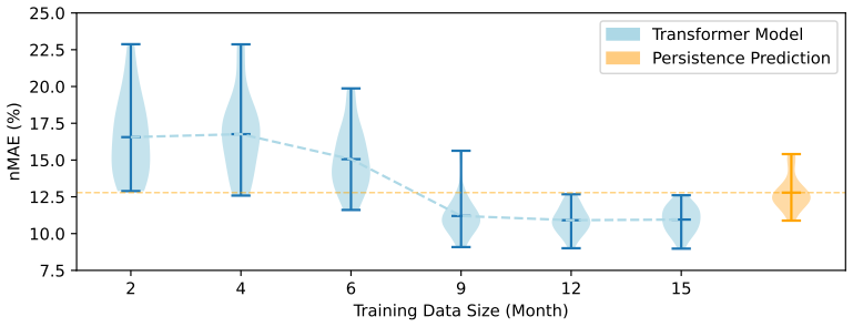
The central claim is that for day-ahead load forecasting in energy communities, deep learning models are not universally superior to simple benchmarks. On the paper's test setup (Q4 2013, 20 virtual communities per configuration), persistence forecasting has lower nMAE than LSTM, xLSTM, and Transformer models for training windows of 2, 4, and 6 months; the deep models only overtake persistence once 9 to 12 months of training data are available, and the gain plateaus around 12 months. Transfer learning from publicly available synthetic profiles (German standard load profiles) improves the deep models' nMAE by 1.97 percentage points on average in the two-month data setting, but the benefit fades with more data. In the financial case study, a mixed-integer linear program scheduling a shared community battery under a day-ahead real-time price produces average cost savings of 8.06% for the best deep learning model and 8.01% for KNN at 50 households, with all models converging toward 8.3–8.4% at 100 households. The authors conclude that simple, robust models are competitive and often preferable for newly formed or data-scarce communities.
Load-bearing premise
The six-month crossover is measured on a single test season, Q4 2013; the paper assumes that this quarter represents the whole year, so if winter or summer load patterns shift the crossover, the threshold would move.
Editorial extensions
If this is right
- Energy communities with less than six months of operation should plan on persistence forecasting for model-predictive control; deep learning only pays off after roughly nine months of collected data.
- Public synthetic load profiles are a viable pretraining source for data-scarce communities, cutting nMAE by about 2 percentage points when only two months of target data exist.
- A simple KNN forecaster can capture nearly all the financial value of deep learning in a battery storage optimization, at a fraction of the complexity.
- Transformer forecast accuracy is stable down to roughly 200 parameters, so model complexity can be reduced substantially for edge deployments without sacrificing accuracy.
- Forecast error and its financial impact shrink as community aggregation grows; at 100 households all tested forecasters yield 8.28–8.39% savings.
Reading between the lines
- The six-month crossover was tested on an autumn quarter only; an obvious extension is to repeat the training-size sweep on winter, spring, and summer test sets to see whether the threshold is seasonal.
- Because the financial case study uses a day-ahead real-time price, the price signal itself carries much of the scheduling information; under more prediction-sensitive objectives, such as peak-load minimization or self-sufficiency, the gap between KNN and deep learning could widen.
- The transfer-learning recipe could be tested across countries and climates; the 1.97 percentage point gain from German synthetic profiles on UK data suggests larger gains or losses if source and target diverge more.
- The same benchmark grid could be run with probabilistic forecasts (quantiles or intervals) since the MILP objective and the 15% grid-purchase constraint may respond differently to error distributions, not just mean error.
Signed reviews
Editorial analysis
A structured set of objections, weighed in public.
Referee Report
Summary. The paper benchmarks three deep-learning load forecasters (LSTM, xLSTM, Transformer) against persistence and KNN for day-ahead forecasting of virtual energy communities built from 4,500 London smart-meter profiles. It reports three main results: persistence beats all deep-learning models when training data are below six months; transfer learning from German synthetic load profiles improves mean nMAE by 1.97 percentage points when only two months of target data are available; and in a MILP battery-storage case study, KNN achieves financial savings (8.01% for 50 households) nearly identical to the best deep-learning model (8.06%). The paper also analyzes sensitivity to community size and model size, and it releases code and data for reproducibility.
Significance. If the headline threshold holds, the paper provides a practically useful rule for model selection in new energy communities, and it is one of the few studies that combine a broad benchmark, transfer learning, and an economic optimization case study in one framework. The transfer-learning figure is concrete and can be verified directly from Tables A.1 and A.2, and the KNN-versus-deep-learning savings comparison in Table A.3 is a valuable, credible result. The central limitation is that the persistence-beats-deep-learning threshold is established on a single test season, so the practical significance of the main claim depends on closing this seasonal-generalizability gap.
major comments (1)
- [Section 2.3, Fig. 8, Appendix B] The central claim that persistence outperforms LSTM, xLSTM, and Transformer with less than six months of training data is established only on the Q4 2013 test period. Appendix B reports results for Q1-Q3 test quarters, but those runs use a fixed three-quarter training window of about nine months and, for Q1, Q2, and Q3, the training set includes future quarters (Q2-Q4, Q3-Q4, and Q4 of 2013, respectively), which the authors themselves describe as unrealistic. These runs therefore do not test whether the six-month threshold also holds in other seasons. Please either run the 2/4/6-month training-size sweep for other test quarters using only past data, or qualify the threshold claim as specific to the Q4 test period.
minor comments (8)
- [Section 3.2, Fig. 8] The sentence 'with nine months of training data or more, the deep learning models outperform persistent prediction, with a difference in nMAE ranging from 1.8 percentage points to 2.0 percentage points' is not supported by Table A.1: at nine months the differences from persistence (12.79%) are 1.23, 1.23, and 1.59 percentage points for xLSTM, LSTM, and Transformer, respectively. The 1.8-2.0 range appears only at 12-15 months.
- [Abstract and Conclusions] The abstract says 'less than six months' while the Conclusions say 'six months or less'; since the 6-month rows in Tables A.1 and A.2 still favor persistence, please choose one formulation and use it consistently.
- [Table A.1] The xLSTM entries for 0.1k and 0.2k model sizes are marked '-' although Table C.5 lists configurations for these sizes; please clarify whether these runs were omitted or failed to converge.
- [Section 2.4] The perfect-prediction scenario omits Eq. 7 while all forecast-based scenarios include it, so the savings gap between perfect and imperfect forecasts is not solely attributable to forecast quality; please state this explicitly when interpreting the perfect-prediction baseline.
- [Figure 9] The caption says 'The column shows the mean over 20 ECs' but the figure appears to display distributions; please specify exactly what the boxes, whiskers, and markers represent.
- [Section 3.2, Table A.1] For the decisive 6-month comparison, please report paired confidence intervals or a test statistic, because the LSTM-versus-persistence difference (13.46% vs. 12.79%) is small relative to the reported standard deviations.
- [Introduction, Contribution 2 and Section 2.2.2] Contribution 2 calls the transfer-learning approach 'novel', but Section 2.2.2 states that the same approach was already applied in reference [25]; please clarify what is genuinely new in the present application.
- [Conclusions] The 10-household, 120 kWh case referenced in the Conclusions is not a separate row in Table A.4; adding a note that this configuration corresponds to the 10-household row of Table A.3 would prevent reader confusion.
Circularity Check
No significant circularity: the paper is an empirical benchmark whose forecasts, error metrics, and MILP savings are measured from data rather than derived from the assumptions being tested.
full rationale
The paper's central claims—that persistence beats deep learning below six months of training data, that transfer learning from synthetic profiles helps with two months of data, and that KNN gives nearly the same battery cost savings as deep learning—are all empirical measurements on held-out test data. No equation in the paper defines a prediction in terms of the quantity it is claimed to predict: nMAE is normalized by the measured mean load (Eq. 2), the MILP objective (Eq. 3) minimizes costs given forecasted load, and the reported savings compare optimized grid costs against an unoptimized baseline. The only self-referential element is building on the authors' own prior transfer-learning study [25], but the present multi-model evaluation is an independent re-measurement that does not rely on [25] for its conclusions. Appendix B's acknowledged use of future data as training for some seasonal test quarters is a data-split limitation (the authors themselves call it unrealistic), not a circularity; it weakens the seasonal generalizability of the persistence threshold but does not make any result equivalent to its own input. The persistence-vs-deep-learning threshold is a direct comparison of forecast errors, with no fitted parameter renamed as a prediction, and no load-bearing self-citation chain. Therefore no circular step can be exhibited, and the appropriate score is 0.
Assumptions & free parameters
free parameters (6)
- KNN number of neighbors k =
40
- Baseline model size =
5,000 parameters
- Lagged load lags =
1, 2, and 3 weeks
- BESS capacity per household =
12 kWh
- Minimum grid purchase fraction =
0.15
- Round-trip efficiency =
85% (eta_ch = eta_dis = 92.2%)
assumptions (6)
- domain assumption The 20 randomly sampled household subsets for each community size are representative of real energy communities.
- domain assumption The UK Power Networks smart meter data and Meteostat weather data are accurate and complete.
- domain assumption The MILP formulation (Eqs. 3-22) correctly models a community battery under a real-time price tariff, including the 15% grid-purchase constraint.
- domain assumption Synthetic German load profiles from demandlib are a valid pretraining source for UK household load patterns, despite country differences.
- domain assumption The feature set (datetime, holiday, lagged load, past weather) is sufficient for day-ahead load forecasting.
- domain assumption Q4 2013 is representative of year-round forecasting difficulty for the training-size threshold.
Cite this review
Pith. "Pith review of Load Forecasting for Households and Energy Communities: Are Deep Learning Models Worth the Effort?." pith.science (2026). https://pith.science/paper/CMUT5EVZ
@misc{pith2026250105000,
  author       = {Pith},
  title        = {Pith review of: Load Forecasting for Households and Energy Communities: Are Deep Learning Models Worth the Effort?},
  year         = {2026},
  howpublished = {\url{https://pith.science/paper/CMUT5EVZ}},
  note         = {Machine review of arXiv:2501.05000}
}
read the original abstract
Energy communities (ECs) play a key role in enabling local demand shifting and enhancing self-sufficiency, as energy systems transition toward decentralized structures with high shares of renewable generation. To optimally operate them, accurate short-term load forecasting is essential, particularly for implementing demand-side management strategies. With the recent rise of deep learning methods, data-driven forecasting has gained significant attention, however, it remains insufficiently explored in many practical contexts. Therefore, this study evaluates the effectiveness of state-of-the-art deep learning models-including LSTM, xLSTM, and Transformer architectures-compared to traditional benchmarks such as K-Nearest Neighbors (KNN) and persistence forecasting, across varying community size, historical data availability, and model complexity. Additionally, we assess the benefits of transfer learning using publicly available synthetic load profiles. On average, transfer learning improves the normalized mean absolute error by 1.97 percentage points when only two months of training data are available. Interestingly, for less than six months of training data, simple persistence models outperform deep learning architectures in forecast accuracy. The practical value of improved forecasting is demonstrated using a mixed-integer linear programming optimization for ECs with a shared battery energy storage system. For an energy community with 50 households, the most accurate deep learning model achieves an average reduction in financial energy costs of 8.06%. Notably, a simple KNN approach achieves average savings of 8.01%, making it a competitive and robust alternative. All implementations are publicly available to facilitate reproducibility. These findings offer actionable insights for ECs, and they highlight when the additional complexity of deep learning is warranted by performance gains.
Figures


Figures from the paper (10 more)




Reference graph
Works this paper leans on
-
[1]
European Commission, Clean energy for all Europeans, Publications Office of the European Union, 2019. doi:10.2833/9937
doi:10.2833/9937 2019
-
[2]
P. Ponnaganti, R. Sinha, J. R. Pillai, B. Bak-Jensen, Flexibility provi- sions through local energy communities: A review, Next Energy 1 (2) (2023) 100022. doi:10.1016/j.nxener.2023.100022
arXiv 2023
-
[3]
S. Van Der Stelt, T. AlSkaif, W. Van Sark, Techno-economic analysis of household and community energy storage for residential prosumers with smart appliances, Applied Energy 209 (2018) 266–276. doi:10.1016/ j.apenergy.2017.10.096
work page 2018
-
[4]
D. Mariano-Hern´ andez, L. Hern´ andez-Callejo, A. Zorita-Lamadrid, O. Duque-P´ erez, F. S. Garc ´ ıa, A review of strategies for building energy 29 Table C.5: Configuration of the xLSTM, LSTM, and Transformer of all model sizes. Note that the reported parameter counts are approximate, as slight variations arise due to architectural differences between mo...
arXiv 2021
-
[5]
C. Srithapon, D. M ˚ ansson, Predictive control and coordination for en- ergy community flexibility with electric vehicles, heat pumps and ther- mal energy storage, Applied Energy 347 (2023) 121500. doi:10.1016/ j.apenergy.2023.121500
arXiv 2023
- [6]
-
[7]
K. M. Powell, A. Sriprasad, W. J. Cole, T. F. Edgar, Heating, cooling, and electrical load forecasting for a large-scale district energy system, Energy 74 (2014) 877–885. doi:10.1016/j.energy.2014.07.064
-
[8]
H. Yu, F. Zhong, Y. Du, X. Xie, Y. Wang, X. Zhang, S. Huang, Short- term cooling and heating loads forecasting of building district energy system based on data-driven models, Energy and Buildings 298 (2023) 113513. doi:10.1016/j.enbuild.2023.113513
arXiv 2023
Show all 43 references
-
[9]
Royal, S
E. Royal, S. Bandyopadhyay, A. Newman, Q. Huang, P. C. Tabares- Velasco, A statistical framework for district energy long-term electric load forecasting, Applied Energy 384 (2025) 125445. doi:10.1016/j. apenergy.2025.125445
2025
-
[10]
Peterssen, M
F. Peterssen, M. Schlemminger, C. Lohr, R. Niepelt, R. Hanke- Rauschenbach, R. Brendel, Impact of forecasting on energy system optimization, Advances in Applied Energy 15 (2024) 100181. doi: 10.1016/j.adapen.2024.100181
2024
-
[11]
Wazirali, E
R. Wazirali, E. Yaghoubi, M. S. S. Abujazar, R. Ahmad, A. H. Vak- ili, State-of-the-art review on energy and load forecasting in micro- grids using artificial neural networks, machine learning, and deep learn- ing techniques, Electric power systems research 225 (2023) 109792. ...
2023
-
[12]
Seiler, L
V. Seiler, L. Moosbrugger, G. Huber, P. Kepplinger, Assessing model predictive control for energy communities’ flexibilities, in: Intelli- 31 gente Energie-und Klimastrategien: Energie-Geb¨ aude-Umwelt, no. 30, Holzhausen, 2024. doi:10.57739/978-3-903207-89-9
2024 doi
-
[13]
W. Kong, Z. Y. Dong, Y. Jia, D. J. Hill, Y. Xu, Y. Zhang, Short-term residential load forecasting based on LSTM recurrent neural network, IEEE Transactions on Smart Grid 10 (1) (2019) 841–851.doi:10.1109/ TSG.2017.2753802
2019
-
[14]
Pallonetto, C
F. Pallonetto, C. Jin, E. Mangina, Forecast electricity demand in com- mercial building with machine learning models to enable demand re- sponse programs, Energy and AI 7 (2022) 100121. doi:10.1016/j. egyai.2021.100121
2022
-
[15]
Semmelmann, M
L. Semmelmann, M. Hertel, K. J. Kircher, R. Mikut, V. Hagen- meyer, C. Weinhardt, The impact of heat pumps on day-ahead en- ergy community load forecasting, Applied Energy 368 (2024) 123364. doi:10.1016/j.apenergy.2024.123364
2024
-
[16]
P. Ran, K. Dong, X. Liu, J. Wang, Short-term load forecasting based on ceemdan and transformer, Electric Power Systems Research 214 (2023) 108885. doi:10.1016/j.epsr.2022.108885
2023
-
[17]
Z. Zhao, C. Xia, L. Chi, X. Chang, W. Li, T. Yang, A. Y. Zomaya, Short-term load forecasting based on the transformer model, information 12 (12) (2021) 516. doi:10.3390/info12120516
2021 doi
-
[18]
B. Fang, L. Xu, Y. Luo, Z. Luo, W. Li, A method for short-term electric load forecasting based on the fmlp-itransformer model, Energy Reports 12 (2024) 3405–3411. doi:10.1016/j.egyr.2024.09.023
2024 doi
-
[19]
J. Gao, Y. Chen, W. Hu, D. Zhang, An adaptive deep-learning load forecasting framework by integrating transformer and domain knowl- edge, Advances in Applied Energy 10 (2023) 100142. doi:10.1016/j. adapen.2023.100142
2023
-
[20]
L’Heureux, K
A. L’Heureux, K. Grolinger, M. A. Capretz, Transformer-based model for electrical load forecasting, Energies 15 (14) (2022) 4993. doi:10. 3390/en15144993
2022
- [21]
-
[22]
Kraus, F
M. Kraus, F. Divo, D. S. Dhami, K. Kersting, xlstm-mixer: Multivariate time series forecasting by mixing via scalar memories, arXiv preprint (2024). doi:10.48550/arXiv.2410.16928
2024 doi
-
[23]
E. Lee, W. Rhee, Individualized short-term electric load forecasting with deep neural network based transfer learning and meta learning, IEEE Access 9 (2021) 15413–15425. doi:10.1109/ACCESS.2021.3053317
2021
-
[24]
Ribeiro, K
M. Ribeiro, K. Grolinger, H. F. ElYamany, W. A. Higashino, M. A. Capretz, Transfer learning with seasonal and trend adjustment for cross- building energy forecasting, Energy and Buildings 165 (2018) 352–363. doi:10.1016/j.enbuild.2018.01.034
2018 doi
-
[25]
Moosbrugger, V
L. Moosbrugger, V. Seiler, G. Huber, P. Kepplinger, Improve load fore- casting in energy communities through transfer learning using open- access synthetic profiles, in: 2024 IEEE 8th Forum on Research and Technologies for Society and Industry Innovation (RTSI), IEEE, 2024, pp...
-
[26]
M. G. Pinheiro, S. C. Madeira, A. P. Francisco, Short-term electric- ity load forecasting—a systematic approach from system level to sec- ondary substations, Applied Energy 332 (2023) 120493. doi:10.1016/ j.apenergy.2022.120493
2023
-
[27]
Energy Research Centre, Vorarlberg University of Applied Sciences, Github repository for load forecasting, https://github.com/erc-fhv/ loadforecasting/, accessed: 2024-12-10 (2024)
2024
-
[28]
Y. Chen, D. Zhang, Theory-guided deep-learning for electrical load fore- casting (tgdlf) via ensemble long short-term memory, Advances in Ap- plied Energy 1 (2021) 100004. doi:10.1016/j.adapen.2020.100004
2021
-
[29]
URL https://data.london.gov.uk/dataset/ smartmeter-energy-use-data-in-london-households 33
UK Power Networks, Smartmeter energy consumption data in london households, accessed: 2024-11-20 (2015). URL https://data.london.gov.uk/dataset/ smartmeter-energy-use-data-in-london-households 33
2015
-
[30]
Ceruti, B
A. Ceruti, B. Schachler, C. M¨ oller, F. Maurer, F. Witte, G. Plessmann, H. Huyskens, J. Launer, P. Sch¨ onfeldt, Pyosch, S. Wehkamp, S. Bosch, U. Krien, demandlib: Creating heat and power demand profiles from an- nual values, https://github.com/oemof/demandlib, accessed: 2025...
2016
-
[31]
C. S. Lamprecht, Meteostat Python, accessed on 11 December 2024. URL https://github.com/meteostat/meteostat-python
2024
-
[32]
Ziel, Modeling public holidays in load forecasting: a german case study, Journal of Modern Power Systems and Clean Energy 6 (2) (2018) 191–207
F. Ziel, Modeling public holidays in load forecasting: a german case study, Journal of Modern Power Systems and Clean Energy 6 (2) (2018) 191–207. doi:10.1007/s40565-018-0385-5
2018 doi
- [33]
-
[34]
D. P. Kingma, J. Ba, Adam: A method for stochastic optimization, in: 3rd International Conference on Learning Representations, ICLR 2015, San Diego, CA, USA, May 7-9, 2015, Conference Track Proceedings,
2015
-
[35]
Van Rossum, F
G. Van Rossum, F. L. Drake, Python 3 Reference Manual, CreateSpace, Scotts Valley, CA, 2009
2009
-
[36]
Ansel, E
J. Ansel, E. Yang, H. He, N. Gimelshein, A. Jain, M. e. a. Voznesen- sky, PyTorch 2: Faster Machine Learning Through Dynamic Python Bytecode Transformation and Graph Compilation, in: 29th ACM In- ternational Conference on Architectural Support for Programming Lan- guages and O...
2024
-
[37]
A. Groß, A. Lenders, F. Schwenker, D. A. Braun, D. Fischer, Com- parison of short-term electrical load forecasting methods for differ- ent building types, Energy Informatics 4 (Suppl 3) (2021) 13. doi: 10.1186/s42162-021-00172-6 . 34
2021 doi
-
[38]
Austrian Coordination Office for Energy Communities, Energy commu- nities map, https://energiegemeinschaften.gv.at/landkarte/, ac- cessed: 2024-12-10 (2024)
2024
-
[39]
URL https://www.exaa.at/
EXAA - Die Stromb¨ orse mit f¨ unf Auktionen in AT, DE und NL, accessed on 11 December 2024. URL https://www.exaa.at/
2024
-
[40]
Barbour, D
E. Barbour, D. Parra, Z. Awwad, M. C. Gonz´ alez, Community energy storage: A smart choice for the smart grid?, Applied Energy 212 (2018) 489–497. doi:10.1016/j.apenergy.2017.12.056
2018 doi
-
[41]
W. Cole, A. W. Frazier, C. Augustine, Cost Projections for Utility- Scale Battery Storage: 2021 Update, Tech. Rep. NREL/TP-6A20-79236, National Renewable Energy Lab. (NREL), Golden, CO (United States) (2021). doi:10.2172/1786976
2021 doi
-
[42]
Wohlgenannt, G
P. Wohlgenannt, G. Huber, K. Rheinberger, M. Kolhe, P. Kepplinger, Comparison of demand response strategies using active and passive ther- mal energy storage in a food processing plant, Energy Reports 12 (2024) 226–236. doi:10.1016/j.egyr.2024.06.022. 35
2024 doi
- [2015]
Reviewed August 10, 2026 · model on record in the stance chip above.
Discussion (0). Continue with ORCID to comment.